25 Advanced Pandas Functions People Are Using Without Telling You | by Bex T. | Sep, 2022

ExcelWriter, factorize, explode, squeeze, T, mask, idxmax, clip, …

“I wish I could do this operation in Pandas….”

Well, chances are, you can!

Pandas is so vast and deep that it enables you to execute virtually any tabular manipulation you can think of. However, this vastness sometimes comes at a disadvantage.

Many elegant, advanced features that solve rare edge cases, and unique scenarios are lost in the documentation, shadowed by the more frequently used ones.

This article aims to rediscover those features and show you that Pandas is more awesome than you ever knew.

ExcelWriter is a generic class for creating excel files (with sheets!) and writing DataFrames to them. Let’s say we have these 2:

pipe is one of the best functions for doing data cleaning in a concise, compact manner in Pandas. It allows you to chain multiple custom functions into a single operation.

For example, let’s say you have functions to drop_duplicates, remove_outliers, encode_categoricals that accept their own arguments. Here is how you apply all three in a single operation:

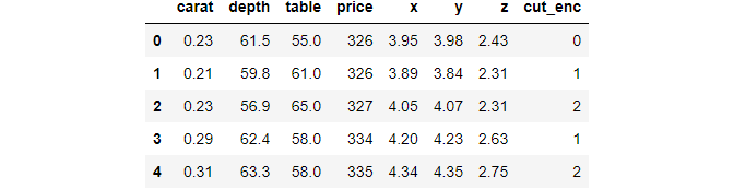
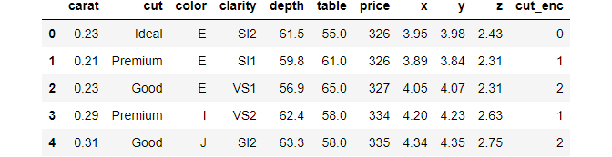
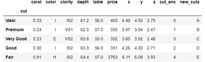
This function is a pandas alternative to Sklearn’s LabelEncoder:

A function with an interesting name is explode. Let’s see an example first and then explain:

The dirty column has two rows where values are recorded as actual lists. You may often see this type of data in surveys as some questions accept multiple answers.

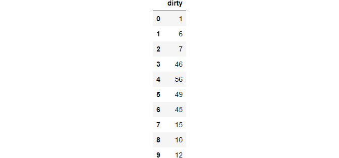
explode takes a cell with an array-like value and explodes it into multiple rows. Set ignore_index to True to keep the ordering of a numeric index.

Another function with a funky name is squeeze and is used in very rare but annoying edge cases.

One of these cases is when a single value is returned from a condition used to subset a DataFrame. Consider this example:

Even though there is just one cell, it is returned as a DataFrame. This can be annoying since you now have to use .loc again with both the column name and index to access the price.

But, if you know squeeze, you don’t have to. The function enables you to remove an axis from a single-cell DataFrame or Series. For example:

>>> subset.squeeze()326

Now, only the scalar is returned. It is also possible to specify the axis to remove:

Note that squeeze only works for DataFrames or Series with single values.

A rather nifty function for boolean indexing numeric features within a range:

All DataFrames have a simple T attribute, which stands for transpose. You may not use it often, but I find it quite useful when displaying DataFrames of the describe method:

>>> boston.describe().T.head(10)

The Boston housing dataset has 30 numeric columns. If you call describe as-is, the DataFrame will stretch horizontally, making it hard to compare the statistics. Taking the transpose will switch the axes so that summary statistics are given in columns.

Did you know that Pandas allows you to style DataFrames?

They have a style attribute, which opens doors to customizations and styles only limited by your HTML and CSS knowledge. I won’t discuss the full details of what you can do with style but only show you my favorite functions:

Above, we are highlighting cells that hold the maximum value of a column. Another cool styler is background_gradient which can give columns a gradient background color based on their values:

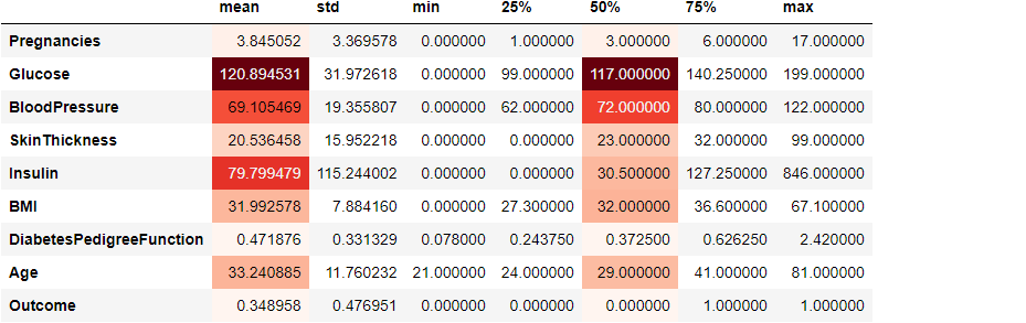
This feature comes especially handy when you are using describe on a table with many columns and want to compare summary statistics. Check out the documentation of the styler here.

Like Matplotlib, pandas has global settings that you can tweak to change the default behaviors:

We all know that pandas has an annoying tendency to mark some columns as object data type. Instead of manually specifying their types, you can use convert_dtypes method which tries to infer the best data type:

A function I use all the time is select_dtypes. I think it is obvious what the function does from its name. It has include and exclude parameters that you can use to select columns including or excluding certain data types.

For example, choose only numeric columns with np.number:

Or exclude them:

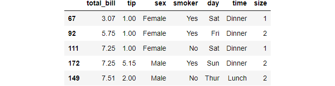
mask allows you to quickly replace cell values where a custom condition is true.

For example, let’s say we have survey data collected from people aged 50–60.

We will treat ages outside the 50–60 range (there are two, 49, and 66) as data entry mistakes and replace them with NaNs.

So, mask replaces values that don’t meet cond with other.

Even though min and max functions are well-known, they have another useful property for some edge-cases. Consider this dataset:

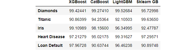
The above fake DataFrame is a point-performance of 4 different gradient boosting libraries on 5 datasets. We want to find the library that performed best at each dataset. Here is how you do it elegantly with max:

Just change the axis to 1, and you get a row-wise max/min.

Sometimes you don’t just want the min/max of a column. You want to see the top N or ~(top N) values of a variable. This is where nlargest and nsmallest comes in handy.

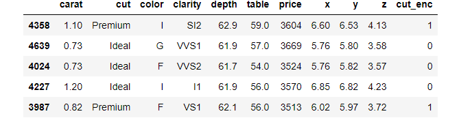
Let’s see the top 5 most expensive and cheapest diamonds:

When you call max or min on a column, pandas returns the value that is largest/smallest. However, sometimes you want the position of the min/max, which is not possible with these functions.

Instead, you should use idxmax/idxmin:

A common operation to find the percentage of missing values is to chain isnull and sum and divide by the length of the array.

But, you can do the same thing with value_counts with relevant arguments:

Outlier detection and removal are common in data analysis.

clip function makes it really easy to find outliers outside a range and replace them with the hard limits.

Let’s go back to the ages example:

This time, we will replace the out-of-range ages with the hard limits of 50 and 60:

>>> ages.clip(50, 60)

Fast and efficient!

These two can be useful when working with time series that have high granularity.

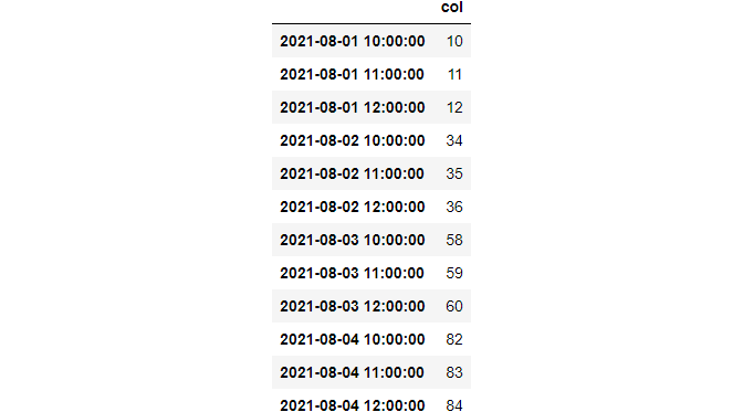
at_time allows you to subset values at a specific date or time. Consider this time series:

Let’s select all rows at 3 PM:

>>> data.at_time("15:00")

Cool, huh? Now, let’s use between_time to select rows within a custom interval:

Note that both functions require a DateTimeIndex, and they only work with times (as in o’clock). If you want to subset within a DateTime interval, use between.

bdate_range is a short-hand function to create TimeSeries indices with business-day frequency:

One of the critical components in time-series analysis is examining the autocorrelation of a variable.

Autocorrelation is the plain-old correlation coefficient, but it is calculated with the lagging version of a time series.

In more detail, the autocorrelation of a time series at lag=k is calculated as follows:

1. The time-series is shifted till k periods:

2. Correlation is calculated between the original tip and each lag_*.

Instead of doing all this manually, you can use the autocorr function of Pandas:

You can read more about the importance of autocorrelation in time-series analysis from this post.

Pandas offers a quick method to check if a given series contains any nulls with hasnans attribute:

These two accessors are much faster alternatives to loc and iloc with a disadvantage. They only allow selecting or replacing a single value at a time:

You should use this function when you want to extract the indices that would sort an array:

It is common knowledge that Pandas enables to use built-in Python functions on dates and strings using accessors like dt or str.

Pandas also has a special category data type for categorical variables as can be seen below:

This function only works with GroupBy objects. Specifically, after grouping, nth returns the nth row from each group:

>>> diamonds.groupby("cut").nth(5)

Even though libraries like Dask and datatable are slowly winning over Pandas with their shiny new features for handling massive datasets, Pandas remains the most widely-used data manipulation tool in the Python data science ecosystem.

The library is a role model for other packages to imitate and improve upon, as it integrates into the modern SciPy stack so well.

Thank you for reading!

ExcelWriter, factorize, explode, squeeze, T, mask, idxmax, clip, …

“I wish I could do this operation in Pandas….”

Well, chances are, you can!

Pandas is so vast and deep that it enables you to execute virtually any tabular manipulation you can think of. However, this vastness sometimes comes at a disadvantage.

Many elegant, advanced features that solve rare edge cases, and unique scenarios are lost in the documentation, shadowed by the more frequently used ones.

This article aims to rediscover those features and show you that Pandas is more awesome than you ever knew.

ExcelWriter is a generic class for creating excel files (with sheets!) and writing DataFrames to them. Let’s say we have these 2:

pipe is one of the best functions for doing data cleaning in a concise, compact manner in Pandas. It allows you to chain multiple custom functions into a single operation.

For example, let’s say you have functions to drop_duplicates, remove_outliers, encode_categoricals that accept their own arguments. Here is how you apply all three in a single operation:

This function is a pandas alternative to Sklearn’s LabelEncoder:

A function with an interesting name is explode. Let’s see an example first and then explain:

The dirty column has two rows where values are recorded as actual lists. You may often see this type of data in surveys as some questions accept multiple answers.

explode takes a cell with an array-like value and explodes it into multiple rows. Set ignore_index to True to keep the ordering of a numeric index.

Another function with a funky name is squeeze and is used in very rare but annoying edge cases.

One of these cases is when a single value is returned from a condition used to subset a DataFrame. Consider this example:

Even though there is just one cell, it is returned as a DataFrame. This can be annoying since you now have to use .loc again with both the column name and index to access the price.

But, if you know squeeze, you don’t have to. The function enables you to remove an axis from a single-cell DataFrame or Series. For example:

>>> subset.squeeze()326

Now, only the scalar is returned. It is also possible to specify the axis to remove:

Note that squeeze only works for DataFrames or Series with single values.

A rather nifty function for boolean indexing numeric features within a range:

All DataFrames have a simple T attribute, which stands for transpose. You may not use it often, but I find it quite useful when displaying DataFrames of the describe method:

>>> boston.describe().T.head(10)

The Boston housing dataset has 30 numeric columns. If you call describe as-is, the DataFrame will stretch horizontally, making it hard to compare the statistics. Taking the transpose will switch the axes so that summary statistics are given in columns.

Did you know that Pandas allows you to style DataFrames?

They have a style attribute, which opens doors to customizations and styles only limited by your HTML and CSS knowledge. I won’t discuss the full details of what you can do with style but only show you my favorite functions:

Above, we are highlighting cells that hold the maximum value of a column. Another cool styler is background_gradient which can give columns a gradient background color based on their values:

This feature comes especially handy when you are using describe on a table with many columns and want to compare summary statistics. Check out the documentation of the styler here.

Like Matplotlib, pandas has global settings that you can tweak to change the default behaviors:

We all know that pandas has an annoying tendency to mark some columns as object data type. Instead of manually specifying their types, you can use convert_dtypes method which tries to infer the best data type:

A function I use all the time is select_dtypes. I think it is obvious what the function does from its name. It has include and exclude parameters that you can use to select columns including or excluding certain data types.

For example, choose only numeric columns with np.number:

Or exclude them:

mask allows you to quickly replace cell values where a custom condition is true.

For example, let’s say we have survey data collected from people aged 50–60.

We will treat ages outside the 50–60 range (there are two, 49, and 66) as data entry mistakes and replace them with NaNs.

So, mask replaces values that don’t meet cond with other.

Even though min and max functions are well-known, they have another useful property for some edge-cases. Consider this dataset:

The above fake DataFrame is a point-performance of 4 different gradient boosting libraries on 5 datasets. We want to find the library that performed best at each dataset. Here is how you do it elegantly with max:

Just change the axis to 1, and you get a row-wise max/min.

Sometimes you don’t just want the min/max of a column. You want to see the top N or ~(top N) values of a variable. This is where nlargest and nsmallest comes in handy.

Let’s see the top 5 most expensive and cheapest diamonds:

When you call max or min on a column, pandas returns the value that is largest/smallest. However, sometimes you want the position of the min/max, which is not possible with these functions.

Instead, you should use idxmax/idxmin:

A common operation to find the percentage of missing values is to chain isnull and sum and divide by the length of the array.

But, you can do the same thing with value_counts with relevant arguments:

Outlier detection and removal are common in data analysis.

clip function makes it really easy to find outliers outside a range and replace them with the hard limits.

Let’s go back to the ages example:

This time, we will replace the out-of-range ages with the hard limits of 50 and 60:

>>> ages.clip(50, 60)

Fast and efficient!

These two can be useful when working with time series that have high granularity.

at_time allows you to subset values at a specific date or time. Consider this time series:

Let’s select all rows at 3 PM:

>>> data.at_time("15:00")

Cool, huh? Now, let’s use between_time to select rows within a custom interval:

Note that both functions require a DateTimeIndex, and they only work with times (as in o’clock). If you want to subset within a DateTime interval, use between.

bdate_range is a short-hand function to create TimeSeries indices with business-day frequency:

One of the critical components in time-series analysis is examining the autocorrelation of a variable.

Autocorrelation is the plain-old correlation coefficient, but it is calculated with the lagging version of a time series.

In more detail, the autocorrelation of a time series at lag=k is calculated as follows:

1. The time-series is shifted till k periods:

2. Correlation is calculated between the original tip and each lag_*.

Instead of doing all this manually, you can use the autocorr function of Pandas:

You can read more about the importance of autocorrelation in time-series analysis from this post.

Pandas offers a quick method to check if a given series contains any nulls with hasnans attribute:

These two accessors are much faster alternatives to loc and iloc with a disadvantage. They only allow selecting or replacing a single value at a time:

You should use this function when you want to extract the indices that would sort an array:

It is common knowledge that Pandas enables to use built-in Python functions on dates and strings using accessors like dt or str.

Pandas also has a special category data type for categorical variables as can be seen below:

This function only works with GroupBy objects. Specifically, after grouping, nth returns the nth row from each group:

>>> diamonds.groupby("cut").nth(5)

Even though libraries like Dask and datatable are slowly winning over Pandas with their shiny new features for handling massive datasets, Pandas remains the most widely-used data manipulation tool in the Python data science ecosystem.

The library is a role model for other packages to imitate and improve upon, as it integrates into the modern SciPy stack so well.

Thank you for reading!