
Block-Recurrent Transformer: LSTM and Transformer Combined | by Nikos Kafritsas | Jul, 2022
A powerful model that combines the best of both worlds
The vanilla Transformer is no longer the all-mighty model that tackles any case in Deep Learning.
In a previous article, we proved that for time series forecasting tasks, Transformers were struggling. That’s why Google created a hybrid Transformer-LSTM model that achieves SOTA results in time series forecasting tasks.
After the hype ended, researchers started focusing on the shortcomings of Transformers. The new research is directed towards leveraging features from other models (CNNs, RNNs, RL models) to strengthen Transformers. A typical example is the new generation of Vision Transformers[1], where they borrow ideas from CNNs.
In March 2022, a Google Research team and the Swiss AI Lab IDSIA proposed a new architecture, called Block-Recurrent Transformer[2].
So, what is the Block-Recurrent Transformer? It is a novel Transformer model that leverages the recurrence mechanism of LSTMs to achieve significant perplexity improvements in language modeling tasks over long-range sequences.
But first, let’s briefly discuss the strengths and shortcomings of Transformers compared to LSTMS. This will help you understand what inspired the researchers to propose the Block-Recurrent Transformer.
The most significant advantages of Transformers are summarized in the following categories:
Parallelism
RNNs implement sequential processing: The input (let’s say sentences) is processed word by word.
Transformers use non-sequential processing: Sentences are processed as a whole, rather than word by word.
This comparison is better illustrated in Figure 1 and Figure 2.
The LSTM requires 8 time-steps to process the sentences, while BERT[3] requires only 2!
Thus, BERT is better able to take advantage of parallelism, provided by modern GPU acceleration.
Note that both illustrations are simplified: We assumed a batch size of 1. Also, we didn’t bother with BERT’s special tokens, the fact that it takes 2 sentences, etc.
Long-term memory
RNNs are forced to compress their learned representation of the input sequence into a single state vector before moving to future tokens.
Also, while LSTMs solved the vanishing gradient issue that vanilla RNNs suffer from, they are still prone to exploding gradients. Thus, they are struggling with longer dependencies.
Transformers, on the other hand, have much higher bandwidth. For example, in the Encoder-Decoder Transformer[4] model, the Decoder can directly attend to every token in the input sequence, including the already decoded. This is depicted in Figure 3:

Better Attention mechanism
The concept of Attention[4] is not new to Transformers. The Google Neural Engine[5](stacked Bi-LSTMs in encoder-decoder topology) back in 2016 was already using Attention.
Recall that Transformers use a special case called Self-Attention: This mechanism allows each word in the input to reference every other word in the input.
Transformers can use large Attention windows (e.g. 512, 1048). Hence, they are very effective at capturing contextual information in sequential data over long ranges.
Next, let’s move to the Transformer shortcomings:
The O(n²) cost of Self-Attention
The biggest issue of Transformers.
There are two main reasons:
- The initial BERT model has a limit of
512tokens. The naive approach to addressing this issue is to truncate the input sentences. - Alternatively, we can create Transformer Models that surpass that limit, making it up to
4096tokens. However, the cost of self-attention is quadratic with respect to the sentence length.
Hence, scalability becomes quite challenging. Numerous ideas have been proposed that restructure the original self-attention mechanism:
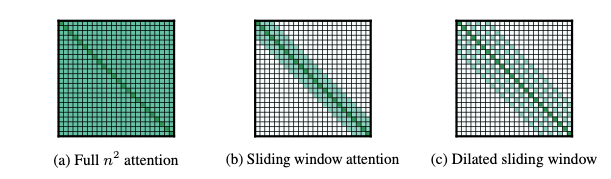
Most of these ideas were introduced by newer-generation models such as Longformer[6] and Transformer XL[7]. These models are optimized for long-form texts and achieve significant improvements.
Nevertheless, the challenge remains: Can we further reduce the computational cost without sacrificing efficiency?
Time series are challenging
While Transformers have dominated the NLP domain, they have limited success with temporal data. But why? Aren’t time series sequential data as well?
- Transformers can better calculate the output of a time-step from long-term history instead of the current input and hidden state. This is less efficient for local temporal dependencies.
- Consequently, short-term memory is equally essential to longer-term memory for time series.
- That’s why Google researchers unveiled a hybrid Deep learning model[1] for Time Series Forecasting: The model uses Attention but also includes an LSTM encoder-decoder stack that plays a significant role in capturing the local temporal dependencies.
- Finally, time series can be multivariate, have static data, and so on. They usually require more special handling.
We won’t focus on the time series aspect in this article. For more information about Deep Learning models for time series, feel free to check this article.
What is the Block-Recurrent Transformer? The Block-Recurrent Transformer is a novel model that revolutionizes the NLP domain.
The main breakthrough of this model is the Recurrent Cell: A modified Transformer layer that works in a recurrent fashion.
Let’s quickly outline the main characteristics and then we will delve deeper into the model’s architecture.
- Block-Level Parallelism: The Recurrent Cell processes tokens in blocks, and all tokens within a block are processed in parallel.
- Large Attention Windows: Since the model breaks the input into blocks, it can use large attention windows (was tested up to
4096tokens). Hence, the Block-Recurrent Transformer belongs to the family of long-range Transformers (like Longformer). - Linear Complexity: Because the Recurrent Cell breaks the input in blocks, the model calculates self-attention block-wise in O(n) time using Sliding Self-Attention.
- More Stable Training: Processing the sequence in blocks can be useful for propagating information and gradients over long distances without causing catastrophic forgetting issues during training.
- Information Diffusion: The Block-Recurrent Transformer operates on a block of state vectors rather than a single vector (like RNNs do). Thus, the model can take full advantage of recurrence and better capture past information.
- Interoperability: The Recurrent Cell can be connected with conventional Transformer layers.
- Modularity: The Recurrent Cells can be stacked horizontally or vertically because the Recurrent Cell can operate in two modes: horizontal (for recurrence) and vertical (for stacking layers). This will become clear in the following section.
- Operational Cost: Adding recurrence is like adding an extra Transformer layer. No extra parameters are introduced.
- Efficiency: The model shows significant improvements compared to other long-range Transformers.
The following two sections will describe in detail the two main components of Block-Recurrent Transformer: The Recurrent Cell architecture and the Sliding Self-Attention with Recurrence.
The backbone of the Block-Recurrent Transformer is the Recurrent Cell.
Note: Don’t get confused by its characterization as ‘Cell’. It’s a fully-fledged Transformer layer, designed to operate in a recurrent way.
The Recurrent Cell receives the following types of input:
- A set of
Wtoken embeddings, withWbeing the block size. - A set of “current state” vectors, called
S.
And the outputs are:
- A set of
Woutput token embeddings. - A set of “next state” vectors.
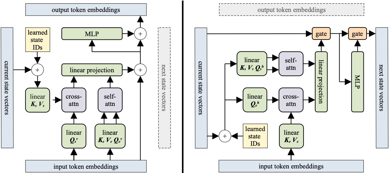
Figure 5 shows the Recurrent Cell architecture. The architecture is quite simple and reuses much of the existing Transformer codebase!
I will explain step-by-step every component shown in Figure 5:
Self-Attention and Cross-Attention
The Block-Recurrent Transformer supports two types of operations: Self-Attention and Cross-Attention. More specifically:
- Self-Attention is performed on keys, values, and queries generated from the same embedding (the
K,V, andQmatrices respectively). - Cross-Attention is performed on queries generated from one embedding, and keys and values generated from another embedding.
If you recall the original Transformer Encoder-Decoder model[4], the Encoder was performing self-attention, while the “encoder-decoder attention” layers in the Decoder performed cross-attention. That’s because the queries come from the previous Decoder layer, while keys and values come from the Encoder output. The Recurrent Cell performs both operations in the same layer. In other words:
The Recurrent Cell does self-attention(encoding) and cross-attention(decoding) in parallel!
Horizontal vs vertical mode
Next, we will focus on the Recurrent Cell architecture, shown in Figure 5. Like I said earlier, the Recurrent Cell operates in two modes:
- Vertical (Stacking): In this mode, the model performs self-attention over the input embeddings and cross-attention over the recurrent states.
- Horizontal (Recurrence): This is exactly the opposite: The model does self-attention over the recurrent states and cross-attention over the input embeddings.
Position bias
You will also notice a square box in Figure 5 called Learned State IDs. Let’s explain what this is and why we need it.
By now, it’s clear that the recurrent state transferred between Recurrent Cells is not a single vector (like RNNs), but a large number of state vectors.
Because the same MLP layer is applied to every state vector (a standard practice), the experimental analysis showed that the state vectors could not differentiate. After a few training epochs, they tend to become identical.
To prevent this issue, the authors added a set of extra learnable “state IDS” to the state vectors. The authors call this functionality position bias. This is analogous to positional encoding, which the vanilla Transformer applies to the input embeddings. The authors of Block-Recurrent Transformer apply this technique to the recurrent state vectors instead, and that’s why they use a different name to avoid confusion.
Positional encoding
The Block-Recurrent Transformer does not apply the conventional positional encoding to the input tokens because they don’t work well for long sequences. Instead, the authors use a famous trick introduced in the T5 architecture [8]: They add positional-relative bias vectors to the self-attention matrix stemming from the input embeddings in the vertical mode. The bias vector is a learned function of the relative distance between keys and queries.
Gate configurations
Another difference between Block-Recurrent Transformer and the other Transformer models is the usage of residual connections.
The authors of Block-Recurrent Transformer tried the following configurations:
- Replacing the residual connections with gates. (This configuration is shown in Figure 5).
- Choosing between a fixed gate and an LSTM gate.
The authors did several experiments to find the optimal configurations. For more details, check the original paper.
The Self-Attention of the Block-Recurrent Transformer is a revolutionary functionality that combines the following concepts:
- The matrix product
QK^TVbecomes ‘linearized’. - Replacing the O(n²) full-attention with O(n) sliding attention.
- Adding recurrence.
The first two concepts have been proposed in related work [6],[9]. Thanks to them, Attention achieves linear cost but loses its potential in very long documents. The Block-Recurrent Transformer combines the first two ideas with recurrence, a concept borrowed from RNNs.
The recurrence mechanism is elegantly integrated inside a Transformer layer and offers dramatically improved results over very long sentences.
We will analyze each concept separately to better understand how the Block-Recurrent Transformer uses Attention.
Linear matrix product
In the Transformer ecosystem, Attention revolves around 3 matrices: The queries Q , the keys K and the valuesV.
As a reminder, the vanilla Attention is given by:
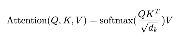
The Block-Recurrent Transformer calculates the Attention score a bit differently: First, the softmax operation is removed. The remaining terms are then re-arranged as Q(K^TV) ( shown in Figure 5) and computed in a linearized manner, according to [9].
Sliding Self-Attention
Given a long sequence of N tokens, a sliding window applies a causal mask so that each token only attends to itself and the previous W tokens. (Remember that W is the block size).
Let’s visualize the attention matrix:
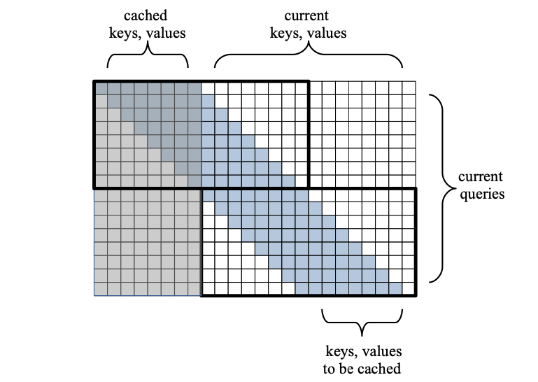
In Figure 6, we have a window size W =8 and sequence length N =16. The first W shaded tokens were computed and cached on the previous training step. The remaining N unshaded tokens come from the current input.
Each token in the input sequence attends to the previous W=8 tokens successively, in a sliding fashion. Therefore, in each row, we have W computations. The height of the matrix is N (the number of tokens in our sentence). Hence, the total cost is O(N*W) instead of the full cost matrix O(N*(W+N)). In other words, the cost with respect to the sequence N is linear instead of quadratic!
So, in our example, Attention is done to two tiles of size Wx2W. Let’s analyze the chain of events:
- In the first attention step, the first
Wtokens of the input sentence will attend to the last cachedWkeysandvaluesfrom the previous sentence. - In the second attention step, the last
Wtokens of our input sentence will attend to the firstWtokens of our input sentence. - This ends our training step and the last
Wkeysandvaluesof the input sentences are cached to be used for the next training step. - By now, you will have noticed the sliding pattern. That’s why we call this mechanism Sliding Self-Attention.
Note: When I say the token X attends to the token Y, we don’t mean the token themselves: I mean the keys, values, and query scores of those respective tokens!
How recurrence helps
As I said earlier, Sliding Self-Attention (the non-recurrent version) was already in use by earlier models [6][7], with a few differences though:
- In the original version, the input sentences were not partitioned into blocks. The models that used the simple Sliding Self-Attention were ingesting the input all at once. This limited the amount of information they could process efficiently.
- The cached keys and values used from the previous training steps are non-differentiable — meaning they are not updated during backpropagation. However, in the recurrent version, the sliding window has an extra advantage because it can backpropagate gradients over multiple blocks.
- The original Sliding Self-Attention model at its topmost layer has a theoretical receptive field of
W*L, whereLrepresents the number of model layers. In the recurrent version, the receptive field is practically unlimited! That’s why the Block-Recurrent Transformer excels in long-range content.
Finally, the Block-Recurrent Transformer was put to the test.
Experimental process
The task was auto-regressive language modeling, where the goal was to predict the next word, given a sentence.
The model was tested on 3 datasets: PG19, arXiv, and Github. All of them contain very long sentences.
The authors tested the Block-Recurrent Transformer and used Transformer XL as a baseline. The Block-Recurrent Transformer was configured in two modes:
- Single Recurrent Mode: The authors used a 12-layer Transformer with recurrence only on layer 10.
- Feedback mode: The same model was used, except this time the 10th layer did not just loop the output to itself: The output of the 10th layer was broadcasted to all the other layers when processing the next block. Hence, layers 1–9 could cross-attend that input, making the model more powerful but computationally more expensive.
Evaluation
The models were evaluated using perplexity — a common metric for language models.
For those who don’t know, perplexity is defined as P=2^L, where L is conventional entropy.
Intuitively, in the context of language modeling, you can think of perplexity in the following way: If the value of perplexity is 30, predicting the next word in the sentence is as uncertain as guessing correctly the result of a 30-sided die. The lower the perplexity, the better.
Results
In general, the Block-Recurrent Transformer significantly outperformed the Transformer XL in terms of both perplexity and speed.
Also, regarding the Block-Recurrent Transformer, the Feedback mode was better than the Single Recurrent Mode. However, the authors conclude that the additional performance does not compensate for the extra complexity.
The paper authors tried various configurations, such as adding or skipping gates. For more information, check the original paper[2].
This article discussed the Block-Recurrent Transformer, a breakthrough paper that leverages the traditional RNN recurrence to increase the Transformer potential in long documents.
I urge you to read the original paper[2], using this article as a companion guide to help your understanding.
Since the paper is very new, the authors have not released any source code, although there are some unofficial implementations on Github.
A powerful model that combines the best of both worlds
The vanilla Transformer is no longer the all-mighty model that tackles any case in Deep Learning.
In a previous article, we proved that for time series forecasting tasks, Transformers were struggling. That’s why Google created a hybrid Transformer-LSTM model that achieves SOTA results in time series forecasting tasks.
After the hype ended, researchers started focusing on the shortcomings of Transformers. The new research is directed towards leveraging features from other models (CNNs, RNNs, RL models) to strengthen Transformers. A typical example is the new generation of Vision Transformers[1], where they borrow ideas from CNNs.
In March 2022, a Google Research team and the Swiss AI Lab IDSIA proposed a new architecture, called Block-Recurrent Transformer[2].
So, what is the Block-Recurrent Transformer? It is a novel Transformer model that leverages the recurrence mechanism of LSTMs to achieve significant perplexity improvements in language modeling tasks over long-range sequences.
But first, let’s briefly discuss the strengths and shortcomings of Transformers compared to LSTMS. This will help you understand what inspired the researchers to propose the Block-Recurrent Transformer.
The most significant advantages of Transformers are summarized in the following categories:
Parallelism
RNNs implement sequential processing: The input (let’s say sentences) is processed word by word.
Transformers use non-sequential processing: Sentences are processed as a whole, rather than word by word.
This comparison is better illustrated in Figure 1 and Figure 2.
The LSTM requires 8 time-steps to process the sentences, while BERT[3] requires only 2!
Thus, BERT is better able to take advantage of parallelism, provided by modern GPU acceleration.
Note that both illustrations are simplified: We assumed a batch size of 1. Also, we didn’t bother with BERT’s special tokens, the fact that it takes 2 sentences, etc.
Long-term memory
RNNs are forced to compress their learned representation of the input sequence into a single state vector before moving to future tokens.
Also, while LSTMs solved the vanishing gradient issue that vanilla RNNs suffer from, they are still prone to exploding gradients. Thus, they are struggling with longer dependencies.
Transformers, on the other hand, have much higher bandwidth. For example, in the Encoder-Decoder Transformer[4] model, the Decoder can directly attend to every token in the input sequence, including the already decoded. This is depicted in Figure 3:
Better Attention mechanism
The concept of Attention[4] is not new to Transformers. The Google Neural Engine[5](stacked Bi-LSTMs in encoder-decoder topology) back in 2016 was already using Attention.
Recall that Transformers use a special case called Self-Attention: This mechanism allows each word in the input to reference every other word in the input.
Transformers can use large Attention windows (e.g. 512, 1048). Hence, they are very effective at capturing contextual information in sequential data over long ranges.
Next, let’s move to the Transformer shortcomings:
The O(n²) cost of Self-Attention
The biggest issue of Transformers.
There are two main reasons:
- The initial BERT model has a limit of
512tokens. The naive approach to addressing this issue is to truncate the input sentences. - Alternatively, we can create Transformer Models that surpass that limit, making it up to
4096tokens. However, the cost of self-attention is quadratic with respect to the sentence length.
Hence, scalability becomes quite challenging. Numerous ideas have been proposed that restructure the original self-attention mechanism:
Most of these ideas were introduced by newer-generation models such as Longformer[6] and Transformer XL[7]. These models are optimized for long-form texts and achieve significant improvements.
Nevertheless, the challenge remains: Can we further reduce the computational cost without sacrificing efficiency?
Time series are challenging
While Transformers have dominated the NLP domain, they have limited success with temporal data. But why? Aren’t time series sequential data as well?
- Transformers can better calculate the output of a time-step from long-term history instead of the current input and hidden state. This is less efficient for local temporal dependencies.
- Consequently, short-term memory is equally essential to longer-term memory for time series.
- That’s why Google researchers unveiled a hybrid Deep learning model[1] for Time Series Forecasting: The model uses Attention but also includes an LSTM encoder-decoder stack that plays a significant role in capturing the local temporal dependencies.
- Finally, time series can be multivariate, have static data, and so on. They usually require more special handling.
We won’t focus on the time series aspect in this article. For more information about Deep Learning models for time series, feel free to check this article.
What is the Block-Recurrent Transformer? The Block-Recurrent Transformer is a novel model that revolutionizes the NLP domain.
The main breakthrough of this model is the Recurrent Cell: A modified Transformer layer that works in a recurrent fashion.
Let’s quickly outline the main characteristics and then we will delve deeper into the model’s architecture.
- Block-Level Parallelism: The Recurrent Cell processes tokens in blocks, and all tokens within a block are processed in parallel.
- Large Attention Windows: Since the model breaks the input into blocks, it can use large attention windows (was tested up to
4096tokens). Hence, the Block-Recurrent Transformer belongs to the family of long-range Transformers (like Longformer). - Linear Complexity: Because the Recurrent Cell breaks the input in blocks, the model calculates self-attention block-wise in O(n) time using Sliding Self-Attention.
- More Stable Training: Processing the sequence in blocks can be useful for propagating information and gradients over long distances without causing catastrophic forgetting issues during training.
- Information Diffusion: The Block-Recurrent Transformer operates on a block of state vectors rather than a single vector (like RNNs do). Thus, the model can take full advantage of recurrence and better capture past information.
- Interoperability: The Recurrent Cell can be connected with conventional Transformer layers.
- Modularity: The Recurrent Cells can be stacked horizontally or vertically because the Recurrent Cell can operate in two modes: horizontal (for recurrence) and vertical (for stacking layers). This will become clear in the following section.
- Operational Cost: Adding recurrence is like adding an extra Transformer layer. No extra parameters are introduced.
- Efficiency: The model shows significant improvements compared to other long-range Transformers.
The following two sections will describe in detail the two main components of Block-Recurrent Transformer: The Recurrent Cell architecture and the Sliding Self-Attention with Recurrence.
The backbone of the Block-Recurrent Transformer is the Recurrent Cell.
Note: Don’t get confused by its characterization as ‘Cell’. It’s a fully-fledged Transformer layer, designed to operate in a recurrent way.
The Recurrent Cell receives the following types of input:
- A set of
Wtoken embeddings, withWbeing the block size. - A set of “current state” vectors, called
S.
And the outputs are:
- A set of
Woutput token embeddings. - A set of “next state” vectors.
Figure 5 shows the Recurrent Cell architecture. The architecture is quite simple and reuses much of the existing Transformer codebase!
I will explain step-by-step every component shown in Figure 5:
Self-Attention and Cross-Attention
The Block-Recurrent Transformer supports two types of operations: Self-Attention and Cross-Attention. More specifically:
- Self-Attention is performed on keys, values, and queries generated from the same embedding (the
K,V, andQmatrices respectively). - Cross-Attention is performed on queries generated from one embedding, and keys and values generated from another embedding.
If you recall the original Transformer Encoder-Decoder model[4], the Encoder was performing self-attention, while the “encoder-decoder attention” layers in the Decoder performed cross-attention. That’s because the queries come from the previous Decoder layer, while keys and values come from the Encoder output. The Recurrent Cell performs both operations in the same layer. In other words:
The Recurrent Cell does self-attention(encoding) and cross-attention(decoding) in parallel!
Horizontal vs vertical mode
Next, we will focus on the Recurrent Cell architecture, shown in Figure 5. Like I said earlier, the Recurrent Cell operates in two modes:
- Vertical (Stacking): In this mode, the model performs self-attention over the input embeddings and cross-attention over the recurrent states.
- Horizontal (Recurrence): This is exactly the opposite: The model does self-attention over the recurrent states and cross-attention over the input embeddings.
Position bias
You will also notice a square box in Figure 5 called Learned State IDs. Let’s explain what this is and why we need it.
By now, it’s clear that the recurrent state transferred between Recurrent Cells is not a single vector (like RNNs), but a large number of state vectors.
Because the same MLP layer is applied to every state vector (a standard practice), the experimental analysis showed that the state vectors could not differentiate. After a few training epochs, they tend to become identical.
To prevent this issue, the authors added a set of extra learnable “state IDS” to the state vectors. The authors call this functionality position bias. This is analogous to positional encoding, which the vanilla Transformer applies to the input embeddings. The authors of Block-Recurrent Transformer apply this technique to the recurrent state vectors instead, and that’s why they use a different name to avoid confusion.
Positional encoding
The Block-Recurrent Transformer does not apply the conventional positional encoding to the input tokens because they don’t work well for long sequences. Instead, the authors use a famous trick introduced in the T5 architecture [8]: They add positional-relative bias vectors to the self-attention matrix stemming from the input embeddings in the vertical mode. The bias vector is a learned function of the relative distance between keys and queries.
Gate configurations
Another difference between Block-Recurrent Transformer and the other Transformer models is the usage of residual connections.
The authors of Block-Recurrent Transformer tried the following configurations:
- Replacing the residual connections with gates. (This configuration is shown in Figure 5).
- Choosing between a fixed gate and an LSTM gate.
The authors did several experiments to find the optimal configurations. For more details, check the original paper.
The Self-Attention of the Block-Recurrent Transformer is a revolutionary functionality that combines the following concepts:
- The matrix product
QK^TVbecomes ‘linearized’. - Replacing the O(n²) full-attention with O(n) sliding attention.
- Adding recurrence.
The first two concepts have been proposed in related work [6],[9]. Thanks to them, Attention achieves linear cost but loses its potential in very long documents. The Block-Recurrent Transformer combines the first two ideas with recurrence, a concept borrowed from RNNs.
The recurrence mechanism is elegantly integrated inside a Transformer layer and offers dramatically improved results over very long sentences.
We will analyze each concept separately to better understand how the Block-Recurrent Transformer uses Attention.
Linear matrix product
In the Transformer ecosystem, Attention revolves around 3 matrices: The queries Q , the keys K and the valuesV.
As a reminder, the vanilla Attention is given by:
The Block-Recurrent Transformer calculates the Attention score a bit differently: First, the softmax operation is removed. The remaining terms are then re-arranged as Q(K^TV) ( shown in Figure 5) and computed in a linearized manner, according to [9].
Sliding Self-Attention
Given a long sequence of N tokens, a sliding window applies a causal mask so that each token only attends to itself and the previous W tokens. (Remember that W is the block size).
Let’s visualize the attention matrix:
In Figure 6, we have a window size W =8 and sequence length N =16. The first W shaded tokens were computed and cached on the previous training step. The remaining N unshaded tokens come from the current input.
Each token in the input sequence attends to the previous W=8 tokens successively, in a sliding fashion. Therefore, in each row, we have W computations. The height of the matrix is N (the number of tokens in our sentence). Hence, the total cost is O(N*W) instead of the full cost matrix O(N*(W+N)). In other words, the cost with respect to the sequence N is linear instead of quadratic!
So, in our example, Attention is done to two tiles of size Wx2W. Let’s analyze the chain of events:
- In the first attention step, the first
Wtokens of the input sentence will attend to the last cachedWkeysandvaluesfrom the previous sentence. - In the second attention step, the last
Wtokens of our input sentence will attend to the firstWtokens of our input sentence. - This ends our training step and the last
Wkeysandvaluesof the input sentences are cached to be used for the next training step. - By now, you will have noticed the sliding pattern. That’s why we call this mechanism Sliding Self-Attention.
Note: When I say the token X attends to the token Y, we don’t mean the token themselves: I mean the keys, values, and query scores of those respective tokens!
How recurrence helps
As I said earlier, Sliding Self-Attention (the non-recurrent version) was already in use by earlier models [6][7], with a few differences though:
- In the original version, the input sentences were not partitioned into blocks. The models that used the simple Sliding Self-Attention were ingesting the input all at once. This limited the amount of information they could process efficiently.
- The cached keys and values used from the previous training steps are non-differentiable — meaning they are not updated during backpropagation. However, in the recurrent version, the sliding window has an extra advantage because it can backpropagate gradients over multiple blocks.
- The original Sliding Self-Attention model at its topmost layer has a theoretical receptive field of
W*L, whereLrepresents the number of model layers. In the recurrent version, the receptive field is practically unlimited! That’s why the Block-Recurrent Transformer excels in long-range content.
Finally, the Block-Recurrent Transformer was put to the test.
Experimental process
The task was auto-regressive language modeling, where the goal was to predict the next word, given a sentence.
The model was tested on 3 datasets: PG19, arXiv, and Github. All of them contain very long sentences.
The authors tested the Block-Recurrent Transformer and used Transformer XL as a baseline. The Block-Recurrent Transformer was configured in two modes:
- Single Recurrent Mode: The authors used a 12-layer Transformer with recurrence only on layer 10.
- Feedback mode: The same model was used, except this time the 10th layer did not just loop the output to itself: The output of the 10th layer was broadcasted to all the other layers when processing the next block. Hence, layers 1–9 could cross-attend that input, making the model more powerful but computationally more expensive.
Evaluation
The models were evaluated using perplexity — a common metric for language models.
For those who don’t know, perplexity is defined as P=2^L, where L is conventional entropy.
Intuitively, in the context of language modeling, you can think of perplexity in the following way: If the value of perplexity is 30, predicting the next word in the sentence is as uncertain as guessing correctly the result of a 30-sided die. The lower the perplexity, the better.
Results
In general, the Block-Recurrent Transformer significantly outperformed the Transformer XL in terms of both perplexity and speed.
Also, regarding the Block-Recurrent Transformer, the Feedback mode was better than the Single Recurrent Mode. However, the authors conclude that the additional performance does not compensate for the extra complexity.
The paper authors tried various configurations, such as adding or skipping gates. For more information, check the original paper[2].
This article discussed the Block-Recurrent Transformer, a breakthrough paper that leverages the traditional RNN recurrence to increase the Transformer potential in long documents.
I urge you to read the original paper[2], using this article as a companion guide to help your understanding.
Since the paper is very new, the authors have not released any source code, although there are some unofficial implementations on Github.
Denial of responsibility! Techno Blender is an automatic aggregator of the all world’s media. In each content, the hyperlink to the primary source is specified. All trademarks belong to their rightful owners, all materials to their authors. If you are the owner of the content and do not want us to publish your materials, please contact us by email – [email protected]. The content will be deleted within 24 hours.