
Classification of Neural Network in TensorFlow
Classification is used for feature categorization, and only allows one output response for every input pattern as opposed to permitting various faults to occur with a specific set of operating parameters. The category that has the greatest output value is chosen by the classification network. When integrated with numerous forms of predictive neural networks in a hybrid system, classification neural networks become incredibly powerful.
What is Artificial Neural Network?
A substantial majority of heavily integrated processing components known as neurons comprise artificial neural networks, which are computational models that were modeled after biological neural networks.
- Pattern recognition or data segmentation are two instances of applications for which an ANN (Artificial Neural network) is configured.
- It is equipped to make sense of enormous or perplexing material.
- It extracts patterns and detects trends that are too subtle for individuals or other computer technologies to grab on.
Activation Function
The weights and the input-output function which are specified for the unit impact how well the ANN (Artificial Neural Network) responds. One of the three categories outlined below best describes this function:
- Linear: The linear units The output activity has a linear relationship with the overall grade output.
- Threshold: Depending on whether the total input is stronger than or lesser than a certain threshold value, the output is set at one of two levels.
- Sigmoid: As the input fluctuates, the output varies continuously but not linearly. Whereas sigmoid units are more roughly related to actual neurons than the threshold or linear units, all three must be considered approximations.
- ReLU: The rectified linear activation function, commonly known as ReLU, is a non-linear or piecewise linear function that, if the input is positive, gives the input directly; if not, it outputs zero.
- Step: The rectified linear activation function, popularly known as ReLU, is a non-linear or piecewise linear function that, if the input is positive, gives the input directly; if not, it gives zero.
- SoftMax: It turns a real number into a probability density that adds to one, with each member in the output vector reflecting the likelihood that the input vector belongs to a given category.
- Hyperbolic/tanh: A potential function that could be utilized as a nonlinear activation function within layers of a neuron is the hyperbolic function. In fact, it has some similarities to the sigmoid activation function. Both resemble each other a lot. Tanh, however, will map inputs to a range from -1 and 1, whereas a sigmoid function will map input parameters to a range of 0 and 1.
Implementation of sigmoid function :
- Perform an operation that uses the sigmoid function.
- To demonstrate this, we used scikit-learn to create a classification example.
- The ‘make_blobs’ function is used to create a dataset with 60 samples and 2 features.
- Perform operations for classification like binary, to display a number of blobs.
Python3
|
|
Output:
Let’s look at a demonstration of categorization:
- Scikit-learn has significant features and the capability to generate data sets for us.
- Then we’ll declare that our data is equivalent to blobs.
- There are only a few blobs that are generated there that we can characterize.
- As a result, this is merely a binary classification issue as we need to generate 100 samples and three blobs from the number of features.
1. Undertake sigmoid function operations, import libraries, and describe blob characteristics for dataframe in order to display the dataframe.
Python3
|
|
Output:

2. To obtain the output of the type of dataframe we are using in this example, employ the type function.
Output:
tuple
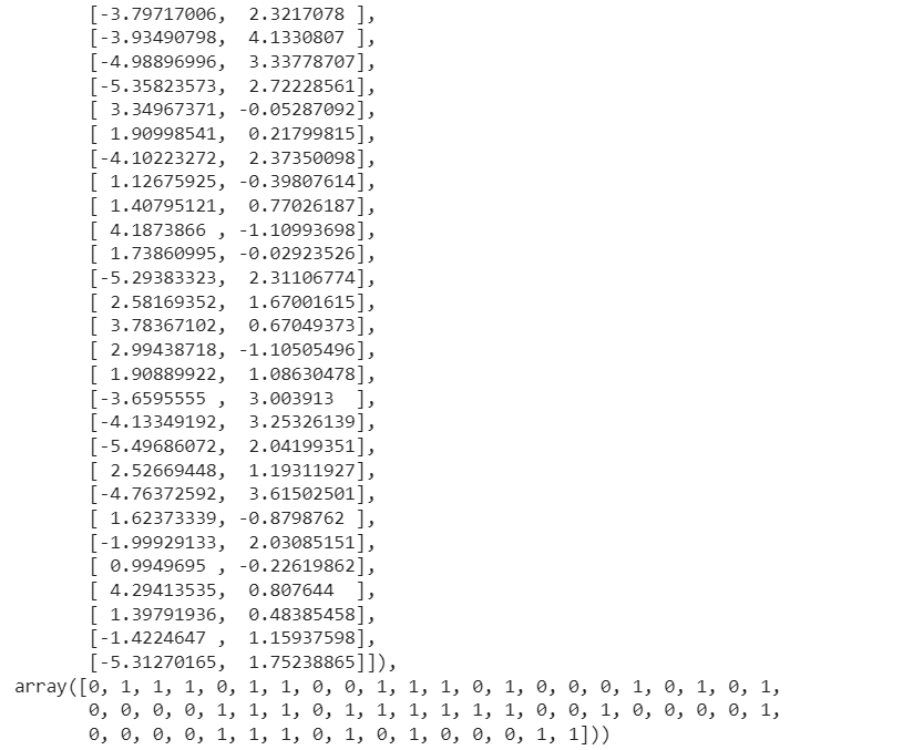
3. Indexing as one to retrieve the outcome of the dataframe’s first index with its values
Output:
array([0, 1, 1, 1, 0, 1, 1, 0, 0, 1, 1, 1, 0, 1, 0, 0, 0, 1, 0, 1, 0, 1,
       0, 0, 0, 0, 1, 1, 1, 0, 1, 1, 1, 1, 1, 1, 0, 0, 1, 0, 0, 0, 0, 1,
       0, 0, 0, 0, 1, 1, 1, 0, 1, 0, 1, 0, 0, 0, 1, 1])
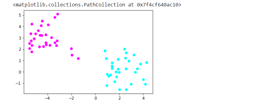
4. Generate the scatterplot and configure the features as well as label and then produce the plots of blobs.
Python3
|
|
Output:
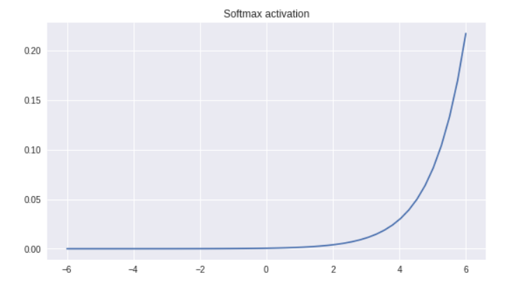
Implementation of SoftMax activation function
- In neural networks, the softmax activation function is very often adopted for multi-class classification methods.
- It is a subtype of activation function that transforms a real-number vector into a probability distribution with a total of one.
- In a multi-class classification issue, the outcome of the softmax function could well be regarded as the likelihood of each class.
- The softmax function is distinguishable, which permits the use of gradient-based optimization techniques, such as stochastic gradient descent.
1. The first and foremost step would be importing the library, then constructing a function to retrieve the softmax function’s output.
Python3
|
|
Output:
array([0.148, 0.804, 0.047])
2. Devise a separate method to perform sum by division and thereafter return the result
Python3
|
|
Output:
array([ 0.249, 1.028, -0.276])
3. Further To acquire the result in the form of an array, construct a variable with the names x1 and x2 and execute the function division sum one which was previously defined.
Python3
|
|
Output:
array([ 0.529, -0.294, 0.765])
Python3
|
|
Output:
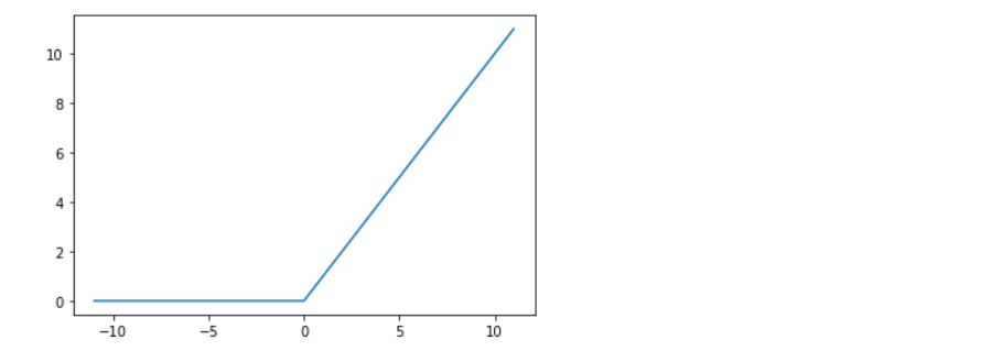
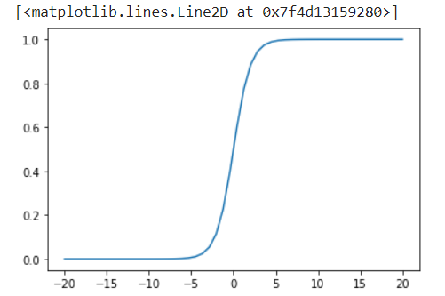
Implementation of rectified linear activation function
- The rectified linear activation function is simple to implement in Python.
- The much more straightforward method is to use the max() function.
- We predict that the procedure will discard whatever favorable input data.
- Intact, however any input parameters of 0.0 or below should be changed to 0.0.
Python3
|
|
Output:
rectified_activation(2.00) gives output as 2.00
rectified_activation(2000.00) gives output as 2000.00
rectified_activation(0.00) gives output as 0.00
rectified_activation(-2.00) gives output as 0.00
rectified_activation(-2000.00) gives output as 0.00
By charting a succession of inputs and computed outputs, we may acquire a notion of the function’s connection among both outputs and inputs.
Python3
|
|
Output:
Implementation of Step activation function
- Neural network models, which are basic neural networks that can categorize inputs based on a set of training instances, may utilize it to categorize responses. It can be challenging to employ the step function in some kinds of neural networks that depend on gradient-based methodologies since it is not distinguishable at the cutoff.
- Instead, the continuous and distinguishable sigmoid function, a version of the step function, is frequently utilized.
- A piecewise function can be used to describe the step function, with a separate function defining the output for each range of input values.
- The step function may be used in conjunction with additional activation functions to build more sophisticated neural networks that are capable of handling a larger variety of tasks.
Python3
|
|
Output:
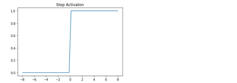
graph of step activation function
Implementation of Hyperbolic/tanh activation function
- Several neural network topologies choose the tanh function because it is a continuous and distinguishable function.
- The tanh function has a symmetric shape around the origin, therefore for negative input parameters, it represents a negative outcome, and for positive input values, it is a positive output.
- The tanh function is much more responsive to changes in the input because it is steeper than that of the sigmoid function in the center of its spectrum.
- The tanh function is frequently employed in recurrent neural networks and may be utilized in neural networks’ convolution neurons as well as their output neurons.
- Since it can aid in preventing the vanishing gradient problem, which can happen in deep neural networks, the hyperbolic activation function is a common option for neural networks.
Python3
|
|
Output:
(400, 400)
Python3
|
|
Output:

graph of hyperbolic activation function
Conclusion:
To summarize, classification neural networks are used to categorize characteristics and only permit one output response for each input pattern. When used in a hybrid system with other prognostic neural networks. The weights and the input-output function of each unit, which might be linear, threshold, sigmoid, RelU, step, Hyperbolic/tanh, or SoftMax, influence the performance of an ANN. For neural network categorization, you may utilize a variety of activation functions.
Classification is used for feature categorization, and only allows one output response for every input pattern as opposed to permitting various faults to occur with a specific set of operating parameters. The category that has the greatest output value is chosen by the classification network. When integrated with numerous forms of predictive neural networks in a hybrid system, classification neural networks become incredibly powerful.
What is Artificial Neural Network?
A substantial majority of heavily integrated processing components known as neurons comprise artificial neural networks, which are computational models that were modeled after biological neural networks.
- Pattern recognition or data segmentation are two instances of applications for which an ANN (Artificial Neural network) is configured.
- It is equipped to make sense of enormous or perplexing material.
- It extracts patterns and detects trends that are too subtle for individuals or other computer technologies to grab on.
Activation Function
The weights and the input-output function which are specified for the unit impact how well the ANN (Artificial Neural Network) responds. One of the three categories outlined below best describes this function:
- Linear: The linear units The output activity has a linear relationship with the overall grade output.
- Threshold: Depending on whether the total input is stronger than or lesser than a certain threshold value, the output is set at one of two levels.
- Sigmoid: As the input fluctuates, the output varies continuously but not linearly. Whereas sigmoid units are more roughly related to actual neurons than the threshold or linear units, all three must be considered approximations.
- ReLU: The rectified linear activation function, commonly known as ReLU, is a non-linear or piecewise linear function that, if the input is positive, gives the input directly; if not, it outputs zero.
- Step: The rectified linear activation function, popularly known as ReLU, is a non-linear or piecewise linear function that, if the input is positive, gives the input directly; if not, it gives zero.
- SoftMax: It turns a real number into a probability density that adds to one, with each member in the output vector reflecting the likelihood that the input vector belongs to a given category.
- Hyperbolic/tanh: A potential function that could be utilized as a nonlinear activation function within layers of a neuron is the hyperbolic function. In fact, it has some similarities to the sigmoid activation function. Both resemble each other a lot. Tanh, however, will map inputs to a range from -1 and 1, whereas a sigmoid function will map input parameters to a range of 0 and 1.
Implementation of sigmoid function :
- Perform an operation that uses the sigmoid function.
- To demonstrate this, we used scikit-learn to create a classification example.
- The ‘make_blobs’ function is used to create a dataset with 60 samples and 2 features.
- Perform operations for classification like binary, to display a number of blobs.
Python3
|
|
Output:
Let’s look at a demonstration of categorization:
- Scikit-learn has significant features and the capability to generate data sets for us.
- Then we’ll declare that our data is equivalent to blobs.
- There are only a few blobs that are generated there that we can characterize.
- As a result, this is merely a binary classification issue as we need to generate 100 samples and three blobs from the number of features.
1. Undertake sigmoid function operations, import libraries, and describe blob characteristics for dataframe in order to display the dataframe.
Python3
|
|
Output:
2. To obtain the output of the type of dataframe we are using in this example, employ the type function.
Output:
tuple
3. Indexing as one to retrieve the outcome of the dataframe’s first index with its values
Output:
array([0, 1, 1, 1, 0, 1, 1, 0, 0, 1, 1, 1, 0, 1, 0, 0, 0, 1, 0, 1, 0, 1,
       0, 0, 0, 0, 1, 1, 1, 0, 1, 1, 1, 1, 1, 1, 0, 0, 1, 0, 0, 0, 0, 1,
       0, 0, 0, 0, 1, 1, 1, 0, 1, 0, 1, 0, 0, 0, 1, 1])
4. Generate the scatterplot and configure the features as well as label and then produce the plots of blobs.
Python3
|
|
Output:
Implementation of SoftMax activation function
- In neural networks, the softmax activation function is very often adopted for multi-class classification methods.
- It is a subtype of activation function that transforms a real-number vector into a probability distribution with a total of one.
- In a multi-class classification issue, the outcome of the softmax function could well be regarded as the likelihood of each class.
- The softmax function is distinguishable, which permits the use of gradient-based optimization techniques, such as stochastic gradient descent.
1. The first and foremost step would be importing the library, then constructing a function to retrieve the softmax function’s output.
Python3
|
|
Output:
array([0.148, 0.804, 0.047])
2. Devise a separate method to perform sum by division and thereafter return the result
Python3
|
|
Output:
array([ 0.249, 1.028, -0.276])
3. Further To acquire the result in the form of an array, construct a variable with the names x1 and x2 and execute the function division sum one which was previously defined.
Python3
|
|
Output:
array([ 0.529, -0.294, 0.765])
Python3
|
|
Output:
Implementation of rectified linear activation function
- The rectified linear activation function is simple to implement in Python.
- The much more straightforward method is to use the max() function.
- We predict that the procedure will discard whatever favorable input data.
- Intact, however any input parameters of 0.0 or below should be changed to 0.0.
Python3
|
|
Output:
rectified_activation(2.00) gives output as 2.00
rectified_activation(2000.00) gives output as 2000.00
rectified_activation(0.00) gives output as 0.00
rectified_activation(-2.00) gives output as 0.00
rectified_activation(-2000.00) gives output as 0.00
By charting a succession of inputs and computed outputs, we may acquire a notion of the function’s connection among both outputs and inputs.
Python3
|
|
Output:
Implementation of Step activation function
- Neural network models, which are basic neural networks that can categorize inputs based on a set of training instances, may utilize it to categorize responses. It can be challenging to employ the step function in some kinds of neural networks that depend on gradient-based methodologies since it is not distinguishable at the cutoff.
- Instead, the continuous and distinguishable sigmoid function, a version of the step function, is frequently utilized.
- A piecewise function can be used to describe the step function, with a separate function defining the output for each range of input values.
- The step function may be used in conjunction with additional activation functions to build more sophisticated neural networks that are capable of handling a larger variety of tasks.
Python3
|
|
Output:
graph of step activation function
Implementation of Hyperbolic/tanh activation function
- Several neural network topologies choose the tanh function because it is a continuous and distinguishable function.
- The tanh function has a symmetric shape around the origin, therefore for negative input parameters, it represents a negative outcome, and for positive input values, it is a positive output.
- The tanh function is much more responsive to changes in the input because it is steeper than that of the sigmoid function in the center of its spectrum.
- The tanh function is frequently employed in recurrent neural networks and may be utilized in neural networks’ convolution neurons as well as their output neurons.
- Since it can aid in preventing the vanishing gradient problem, which can happen in deep neural networks, the hyperbolic activation function is a common option for neural networks.
Python3
|
|
Output:
(400, 400)
Python3
|
|
Output:
graph of hyperbolic activation function
Conclusion:
To summarize, classification neural networks are used to categorize characteristics and only permit one output response for each input pattern. When used in a hybrid system with other prognostic neural networks. The weights and the input-output function of each unit, which might be linear, threshold, sigmoid, RelU, step, Hyperbolic/tanh, or SoftMax, influence the performance of an ANN. For neural network categorization, you may utilize a variety of activation functions.
Denial of responsibility! Techno Blender is an automatic aggregator of the all world’s media. In each content, the hyperlink to the primary source is specified. All trademarks belong to their rightful owners, all materials to their authors. If you are the owner of the content and do not want us to publish your materials, please contact us by email – [email protected]. The content will be deleted within 24 hours.