
Excel Conditional Formatting (with Examples)
Consider a worksheet that has tens of thousands of rows of data. Simply by looking at the raw data – patterns and trends would be very difficult to spot. Conditional formatting offers a further method of visualizing data and improving worksheet comprehension, much like charts.
What is Conditional Formatting in Excel?
Conditional Formatting is a feature in an Excel spreadsheet. It is used to easily maintain the status of the result. It is most often used as color-based formatting to highlight, emphasize, or differentiate among data and information stored in an Excel spreadsheet.
When it comes to applying alternative forms to data that fits particular criteria, Excel conditional formatting is a highly useful feature. It can make it easier for you to draw attention to the key details in your spreadsheets and quickly identify differences in cell values.
Types/Conditional Formatting Presets
You can use preset rules, including Color scales, Data Bars, Icon Sets, Sort filter, etc. to conditionally format your data, or you can construct your own rules that specify when and how the selected cells should be highlighted.
- Data Bars, Similar to a bar graph, data bars are horizontal bars that are added to each cell
Data Bars
- Color scales alter each cell’s color depending on its value. A two- or three-color gradient is used for each color scale
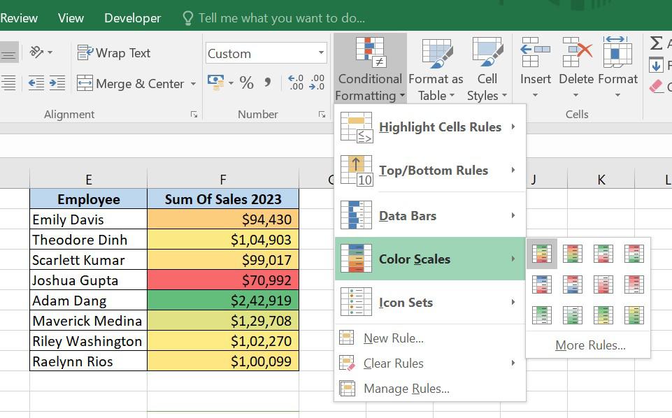
Color scales
- Icon Sets, based on the value of each cell, icon sets assign a distinct icon to each cell.
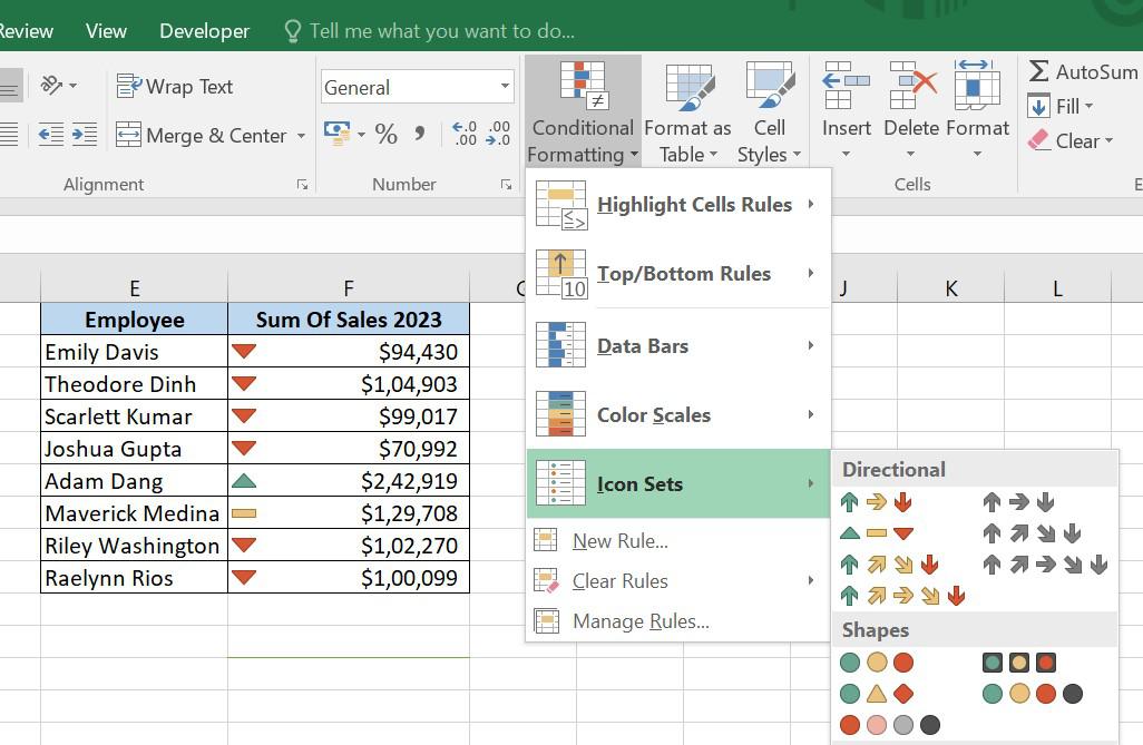
Icon Sets
Where To Find Conditional Formatting in Excel
Conditional formatting is available from Excel 2010 through Excel 365 in the same location.
Home tab > Styles group > Conditional formatting.
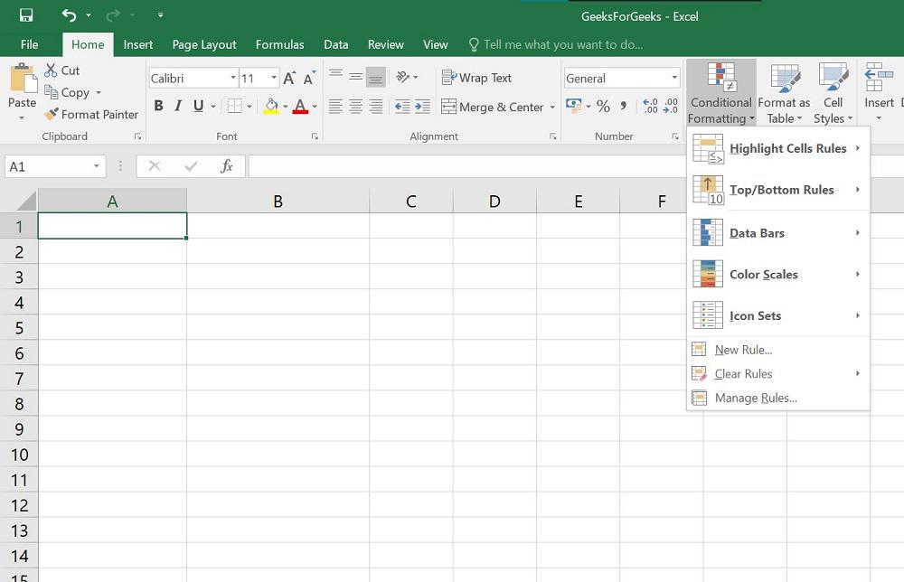
Conditional Formatting in Excel
How to Use Conditional Formatting in Excel
Steps to utilize Excel conditional formatting are as follows:
Step 1. Select the Cells
Select the cells you want to format in the Spreadsheet
Step 2. Click on Conditional Formatting
Click Conditional Formatting, On the Home tab, in the Styles group
Step 3. From a Set of Preset Rules, Pick the Required One
From a set of preset rules, pick the one that best serves your needs
Using Conditional Formatting In Excel
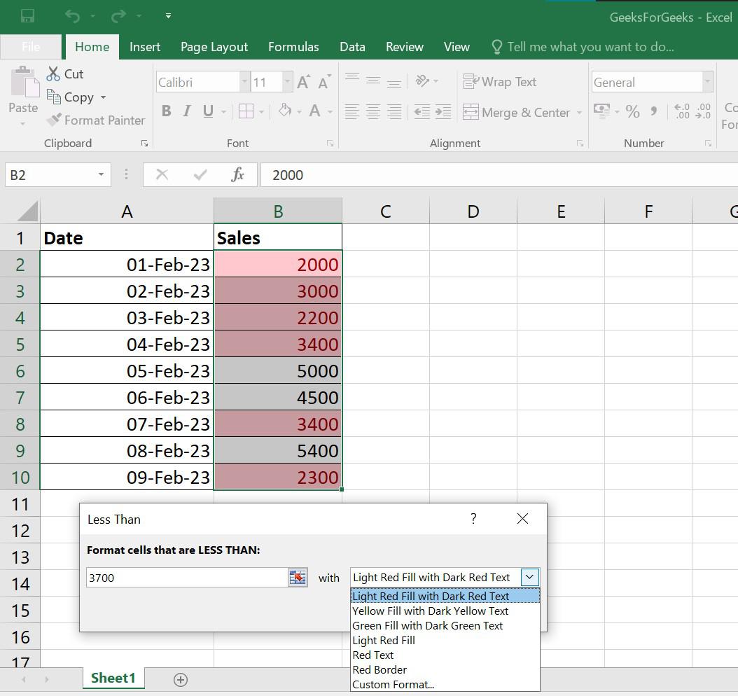
Step 4. Enter the Value and Select the Chosen Format from the Drop-Down List
Enter the value in the box on the left of the dialogue box and select the chosen format from the drop-down list on the right (with Default Light Red Fill with Dark Red Text)
Using Conditional Formatting In Excel
Other rule types that might be appropriate for your data, such as:
- Greater than or equal to
- Between two values
- Text that contains specific words or characters
- Date occurring in a certain range
- Duplicate values
How to Use a Preset Rule with Custom Formatting
You can select any other color for the background, text, or borders of the cells if none of the standard layouts appeals to you. This is how:
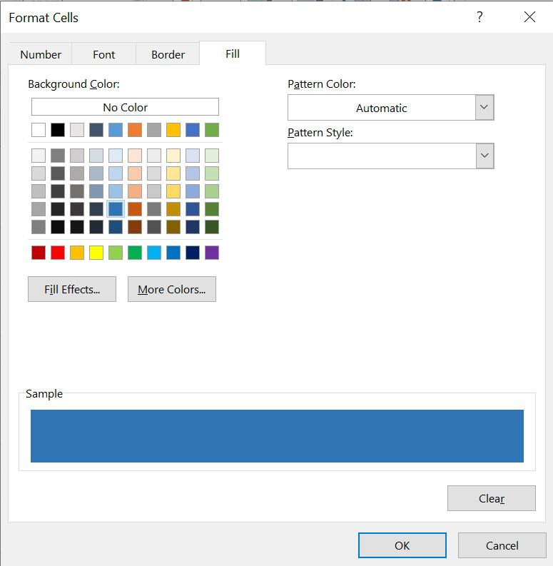
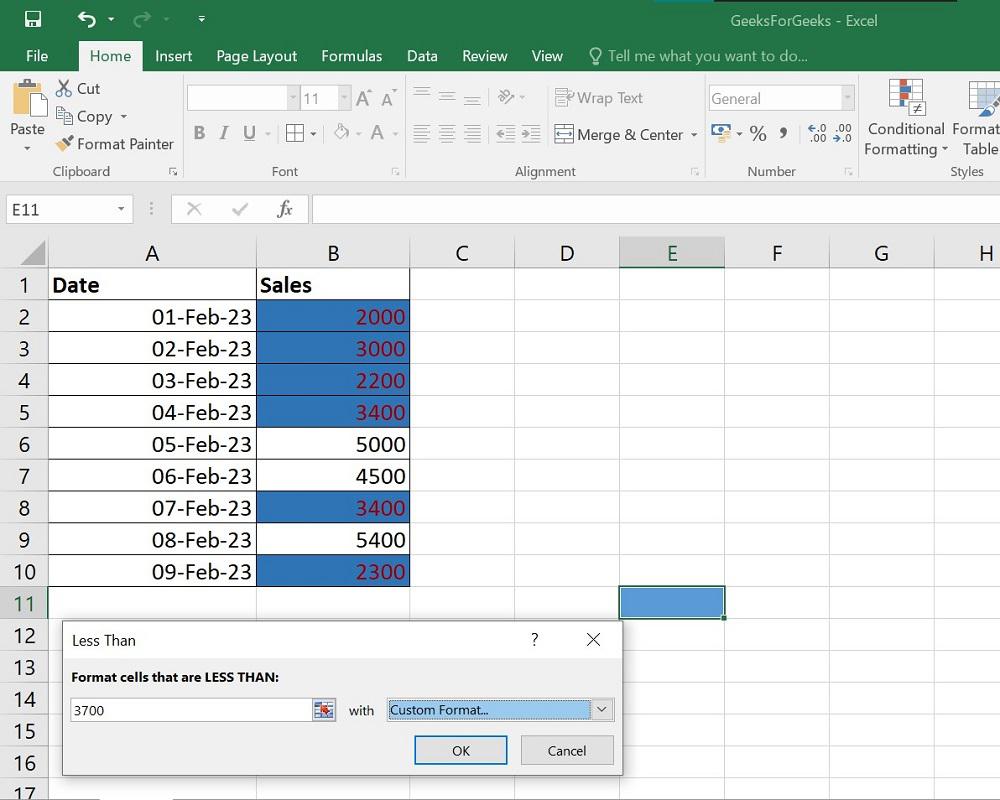
Step 1. Pick Custom Format, In the preset rule dialogue box, from the drop-down list on the right
Step 2. Change between the Font, Border, and Fill tabs in the Format Cells dialogue window to select the preferred font style, border style, and background color, respectively, click OK
Custom formatting
Step 3. Click OK to apply the custom formatting of your choice
Custom formatting
How to Create a New Conditional Formatting Rule in Excel
You can create a new Conditional Formatting Rule in Excel from scratch. To do so, follow these steps:
Step 1. Select the cells to be formatted and click Conditional Formatting > New Rule.
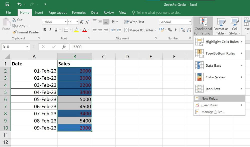
New Conditional Formatting Rule in Excel
Step 2. Select the rule type, in the New Formatting Rule dialog box
New Conditional Formatting Rule in Excel
Step 3. Click the Format button, and choose the color you want to fill.
New Conditional Formatting Rule in Excel
Step 4. Click OK and your New conditional formatting is done!
How to Edit Conditional Formatting Rules in Excel
To make any changes in an already existing Formatting Rule in Excel, follow these steps:
Step 1. Select any cell to which a rule already applies, Click on Manage Rules under Conditional Formatting
Editing Conditional Formatting Rules in Excel
Step 2. This will open the Rules Manager dialog box, select the rule you want to modify, then Click on Edit Rule.
Editing Conditional Formatting Rules in Excel
Step 3. Make the required changes in the Edit Formatting Rule dialogue window, Click on Ok
Excel Conditional Formatting Examples:
Some Scenario-Based Examples of Conditional Formatting in Excel:
Scenario 1. Identifying Duplicates
Steps to identifying duplicate values:
Step 1: Select the cells where you want to identify duplicate values. For example: select the column TOT as shown in the figure.

Step 2: Click on the Conditional Formatting and click on new rules. Now a window appears, select ‘format only unique and duplicate values’ and click on the format.

Step 3: Select the Fill option in the tab and choose the background color and click ok.

Step 4: Now the duplicate values as shown in the figure.

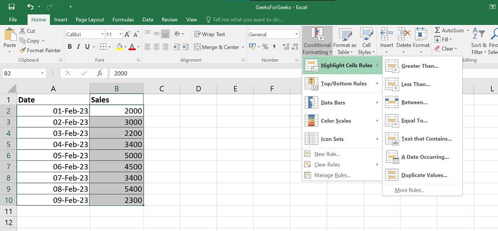
Scenario 2. Cell Highlighting with Value Greater or Less than a Number
Follow the below steps for highlighting cells with a value greater or less than a given number:
Step 1: Select the cells that you want to highlight with Greater or less than a number.

Step 2: Click on the conditional formatting and click on new rules. Now select “Format all cells based on their values“. In the ‘Minimum’ and choose the value you want to identify the lesser values and choose the color. Similarly, In the Maximum and choose the value you want to identify the lesser values and choose the color. And click ok.

Step 3: In the below figure, the values with green color indicate greater values and the values with red color indicate fewer values.

Scenario 3. Highlighting Top or Bottom N Items
To highlight the top and/or the bottom N items select the cells where you want to highlight top and bottom N items and click on the conditional formatting->Top/bottom cells->Top 10 Items. Choose a value in format cells that rank at the top and choose the format and click ok.
In the below figure, the red color indicates the top 5 values in rank.

How to Copy Excel Conditional Formatting
You won’t need to start over when applying a conditional format you’ve already established to different data. To transfer the current conditional formatting rule(s) to another data collection, just utilize Format Painter.
Step 1. Choose the cell whose conditional formatting you want to duplicate
Step 2. Click on Format Painter under Home
Step 3. Click on the first cell in the range you want to format, then drag the paintbrush down to the last cell to paste the copied formatting
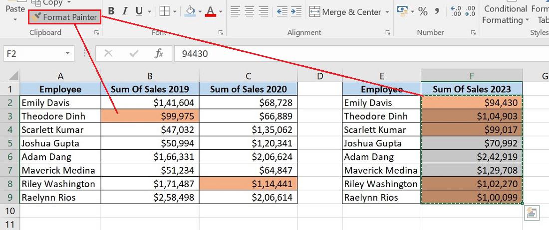
Copy Excel Conditional Formatting
Step 4. To stop using the paintbrush, press Esc.
How to Delete Conditional Formatting Rules
There are two easy ways to delete conditional formatting rules
1. Choose the best choice after selecting the desired cell range and clicking Conditional Formatting > Clear Rules
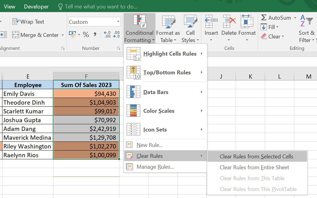
Deleting conditional formatting rules
2. Select the rule and click the Delete Rule button, Under the Conditional Formatting Rules Manager
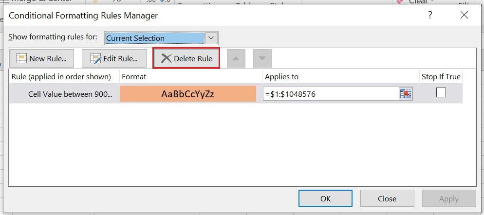
Deleting conditional formatting rules
FAQs on Excel Conditional Formatting
Here are some of the most frequently asked questions on Excel Conditional Formatting
1. What are the 3 conditional formatting options?
Three categories have been established for Conditional Formatting in Excel.
- Similar to a bar graph, Data bars are horizontal bars that are added to each cell
- Color scales alter each cell’s color depending on its value. A two- or three-color gradient is used for each color scale
- Icon Sets, based on the value of each cell, icon sets assign a distinct icon to each cell
2. Can I copy Conditional Formatting to other cells in Excel?
Yes, we can copy Conditional Formatting to other cells in Excel. There are multiple ways to copy the conditional formatting to other cells, such as –
- Simple copy-paste
- Copy and paste conditional formatting only
- Using the format painter
3. How do I remove Conditional Formatting from cells in Excel?
To remove the selected range conditional formatting, please follow the below-mentioned steps:
- Select the range that you want to remove the conditional formatting from
- Click Home > Conditional Formatting > Clear Rules > Clear Rules from Selected Cells
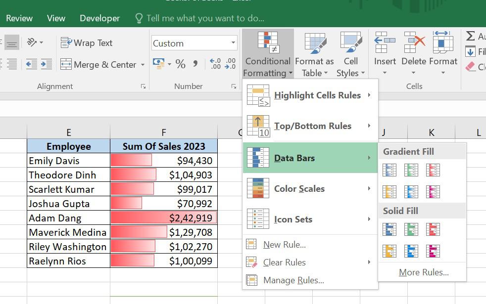
4. Can I use icons or data bars in Conditional Formatting?
Yes, you can use Icons or Data bars in Conditional Formatting in Excel. To use either of these, follow the below steps:
- Select the range that you want to apply the conditional formatting to
- Click on Conditional Formatting on the Home Tab
- Point to Data Bars, and choose from gradient fill or solid fill or Point to Icon sets and choose your desired icons
5. Can I apply Conditional Formatting based on another cell’s value in Excel?
You must use formula if you wish to format an entire row depending on the value of a single cell or apply conditional formatting based on another cell.
Consider a worksheet that has tens of thousands of rows of data. Simply by looking at the raw data – patterns and trends would be very difficult to spot. Conditional formatting offers a further method of visualizing data and improving worksheet comprehension, much like charts.
What is Conditional Formatting in Excel?
Conditional Formatting is a feature in an Excel spreadsheet. It is used to easily maintain the status of the result. It is most often used as color-based formatting to highlight, emphasize, or differentiate among data and information stored in an Excel spreadsheet.
When it comes to applying alternative forms to data that fits particular criteria, Excel conditional formatting is a highly useful feature. It can make it easier for you to draw attention to the key details in your spreadsheets and quickly identify differences in cell values.
Types/Conditional Formatting Presets
You can use preset rules, including Color scales, Data Bars, Icon Sets, Sort filter, etc. to conditionally format your data, or you can construct your own rules that specify when and how the selected cells should be highlighted.
- Data Bars, Similar to a bar graph, data bars are horizontal bars that are added to each cell
Data Bars
- Color scales alter each cell’s color depending on its value. A two- or three-color gradient is used for each color scale
Color scales
- Icon Sets, based on the value of each cell, icon sets assign a distinct icon to each cell.
Icon Sets
Where To Find Conditional Formatting in Excel
Conditional formatting is available from Excel 2010 through Excel 365 in the same location.
Home tab > Styles group > Conditional formatting.
Conditional Formatting in Excel
How to Use Conditional Formatting in Excel
Steps to utilize Excel conditional formatting are as follows:
Step 1. Select the Cells
Select the cells you want to format in the Spreadsheet
Step 2. Click on Conditional Formatting
Click Conditional Formatting, On the Home tab, in the Styles group
Step 3. From a Set of Preset Rules, Pick the Required One
From a set of preset rules, pick the one that best serves your needs
Using Conditional Formatting In Excel
Step 4. Enter the Value and Select the Chosen Format from the Drop-Down List
Enter the value in the box on the left of the dialogue box and select the chosen format from the drop-down list on the right (with Default Light Red Fill with Dark Red Text)
Using Conditional Formatting In Excel
Other rule types that might be appropriate for your data, such as:
- Greater than or equal to
- Between two values
- Text that contains specific words or characters
- Date occurring in a certain range
- Duplicate values
How to Use a Preset Rule with Custom Formatting
You can select any other color for the background, text, or borders of the cells if none of the standard layouts appeals to you. This is how:
Step 1. Pick Custom Format, In the preset rule dialogue box, from the drop-down list on the right
Step 2. Change between the Font, Border, and Fill tabs in the Format Cells dialogue window to select the preferred font style, border style, and background color, respectively, click OK
Custom formatting
Step 3. Click OK to apply the custom formatting of your choice
Custom formatting
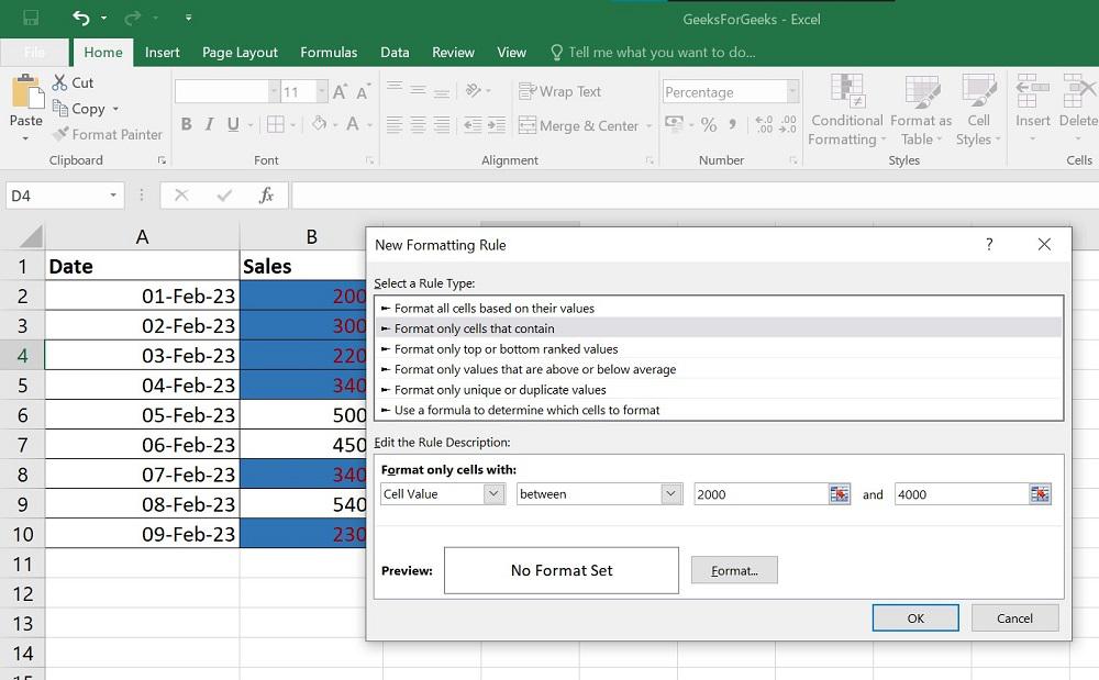
How to Create a New Conditional Formatting Rule in Excel
You can create a new Conditional Formatting Rule in Excel from scratch. To do so, follow these steps:
Step 1. Select the cells to be formatted and click Conditional Formatting > New Rule.
New Conditional Formatting Rule in Excel
Step 2. Select the rule type, in the New Formatting Rule dialog box
New Conditional Formatting Rule in Excel
Step 3. Click the Format button, and choose the color you want to fill.
New Conditional Formatting Rule in Excel
Step 4. Click OK and your New conditional formatting is done!
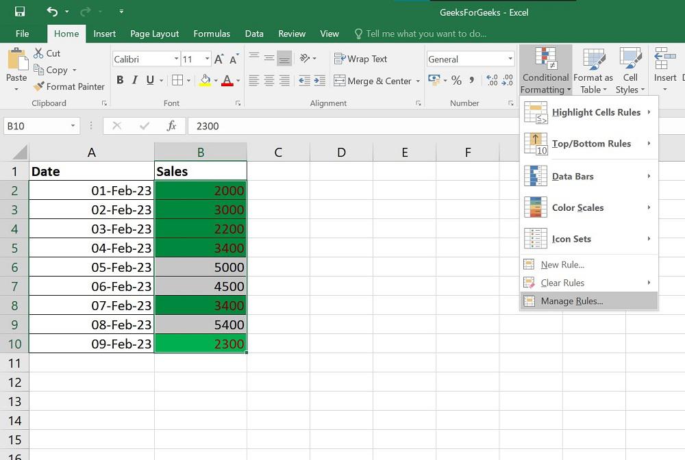
How to Edit Conditional Formatting Rules in Excel
To make any changes in an already existing Formatting Rule in Excel, follow these steps:
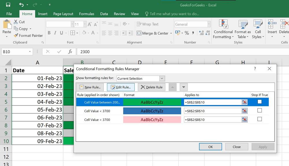
Step 1. Select any cell to which a rule already applies, Click on Manage Rules under Conditional Formatting
Editing Conditional Formatting Rules in Excel
Step 2. This will open the Rules Manager dialog box, select the rule you want to modify, then Click on Edit Rule.
Editing Conditional Formatting Rules in Excel
Step 3. Make the required changes in the Edit Formatting Rule dialogue window, Click on Ok
Excel Conditional Formatting Examples:
Some Scenario-Based Examples of Conditional Formatting in Excel:
Scenario 1. Identifying Duplicates
Steps to identifying duplicate values:
Step 1: Select the cells where you want to identify duplicate values. For example: select the column TOT as shown in the figure.
Step 2: Click on the Conditional Formatting and click on new rules. Now a window appears, select ‘format only unique and duplicate values’ and click on the format.
Step 3: Select the Fill option in the tab and choose the background color and click ok.
Step 4: Now the duplicate values as shown in the figure.
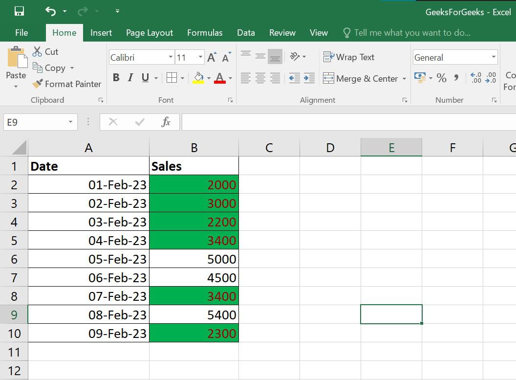
Scenario 2. Cell Highlighting with Value Greater or Less than a Number
Follow the below steps for highlighting cells with a value greater or less than a given number:
Step 1: Select the cells that you want to highlight with Greater or less than a number.
Step 2: Click on the conditional formatting and click on new rules. Now select “Format all cells based on their values“. In the ‘Minimum’ and choose the value you want to identify the lesser values and choose the color. Similarly, In the Maximum and choose the value you want to identify the lesser values and choose the color. And click ok.
Step 3: In the below figure, the values with green color indicate greater values and the values with red color indicate fewer values.
Scenario 3. Highlighting Top or Bottom N Items
To highlight the top and/or the bottom N items select the cells where you want to highlight top and bottom N items and click on the conditional formatting->Top/bottom cells->Top 10 Items. Choose a value in format cells that rank at the top and choose the format and click ok.
In the below figure, the red color indicates the top 5 values in rank.
How to Copy Excel Conditional Formatting
You won’t need to start over when applying a conditional format you’ve already established to different data. To transfer the current conditional formatting rule(s) to another data collection, just utilize Format Painter.
Step 1. Choose the cell whose conditional formatting you want to duplicate
Step 2. Click on Format Painter under Home
Step 3. Click on the first cell in the range you want to format, then drag the paintbrush down to the last cell to paste the copied formatting
Copy Excel Conditional Formatting
Step 4. To stop using the paintbrush, press Esc.
How to Delete Conditional Formatting Rules
There are two easy ways to delete conditional formatting rules
1. Choose the best choice after selecting the desired cell range and clicking Conditional Formatting > Clear Rules
Deleting conditional formatting rules
2. Select the rule and click the Delete Rule button, Under the Conditional Formatting Rules Manager
Deleting conditional formatting rules
FAQs on Excel Conditional Formatting
Here are some of the most frequently asked questions on Excel Conditional Formatting
1. What are the 3 conditional formatting options?
Three categories have been established for Conditional Formatting in Excel.
- Similar to a bar graph, Data bars are horizontal bars that are added to each cell
- Color scales alter each cell’s color depending on its value. A two- or three-color gradient is used for each color scale
- Icon Sets, based on the value of each cell, icon sets assign a distinct icon to each cell
2. Can I copy Conditional Formatting to other cells in Excel?
Yes, we can copy Conditional Formatting to other cells in Excel. There are multiple ways to copy the conditional formatting to other cells, such as –
- Simple copy-paste
- Copy and paste conditional formatting only
- Using the format painter
3. How do I remove Conditional Formatting from cells in Excel?
To remove the selected range conditional formatting, please follow the below-mentioned steps:
- Select the range that you want to remove the conditional formatting from
- Click Home > Conditional Formatting > Clear Rules > Clear Rules from Selected Cells
4. Can I use icons or data bars in Conditional Formatting?
Yes, you can use Icons or Data bars in Conditional Formatting in Excel. To use either of these, follow the below steps:
- Select the range that you want to apply the conditional formatting to
- Click on Conditional Formatting on the Home Tab
- Point to Data Bars, and choose from gradient fill or solid fill or Point to Icon sets and choose your desired icons
5. Can I apply Conditional Formatting based on another cell’s value in Excel?
You must use formula if you wish to format an entire row depending on the value of a single cell or apply conditional formatting based on another cell.
Denial of responsibility! Techno Blender is an automatic aggregator of the all world’s media. In each content, the hyperlink to the primary source is specified. All trademarks belong to their rightful owners, all materials to their authors. If you are the owner of the content and do not want us to publish your materials, please contact us by email – [email protected]. The content will be deleted within 24 hours.