
How Neural Networks Actually Work — Python Implementation (Simplified) | by Kiprono Elijah Koech | May, 2022
Neural Network (NN) is a black box for so many people. We know that it works, but we don’t understand how it works. This article will demystify this belief by working on some examples to show how a neural network really works.
If some terms are not so clear in this article, I have already written two more articles to cover the real basics: article 1 and article 2.
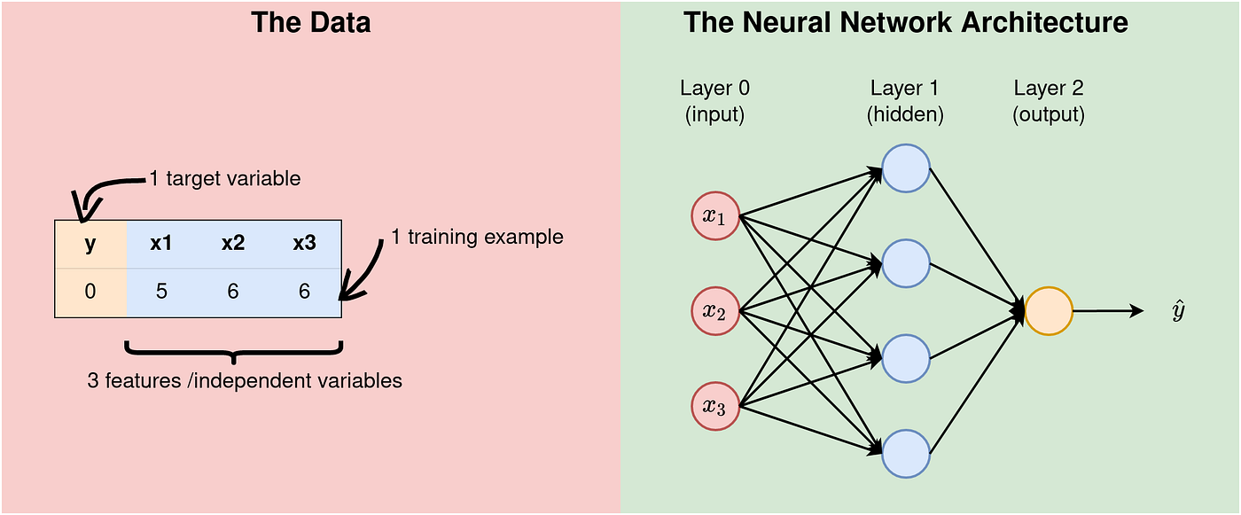
In this first example, let us consider a simple case where we have a dataset of 3 features, a target variable and just one training example (in reality we can never have this kind of data, but, it will make a very good start).
Fact 1: The structure of the data influences the architecture chosen for modelling. In fact, the number of features on the dataset is equal to the number of the neurons in the input layer. In our example, shown in the Figure below, we have 3 features and therefore the input layer of the architecture must have 3 neurons.
The number of hidden layers affects the learning process, and therefore it is chosen based on the application. A network with several hidden layers is called Deep Neural Network (DNN). In this example, we are dealing with a Shallow NN, so to say. We have 3 neurons in the input/first layer, 4 neurons in the hidden layer, and 1 neuron in the output — a 3–4–1 Neural Network.
Let’s set some notations up front so that we can use them going forward without ambiguity. To do this, let us redraw the architecture above to show the parameters and variables used in the NN.
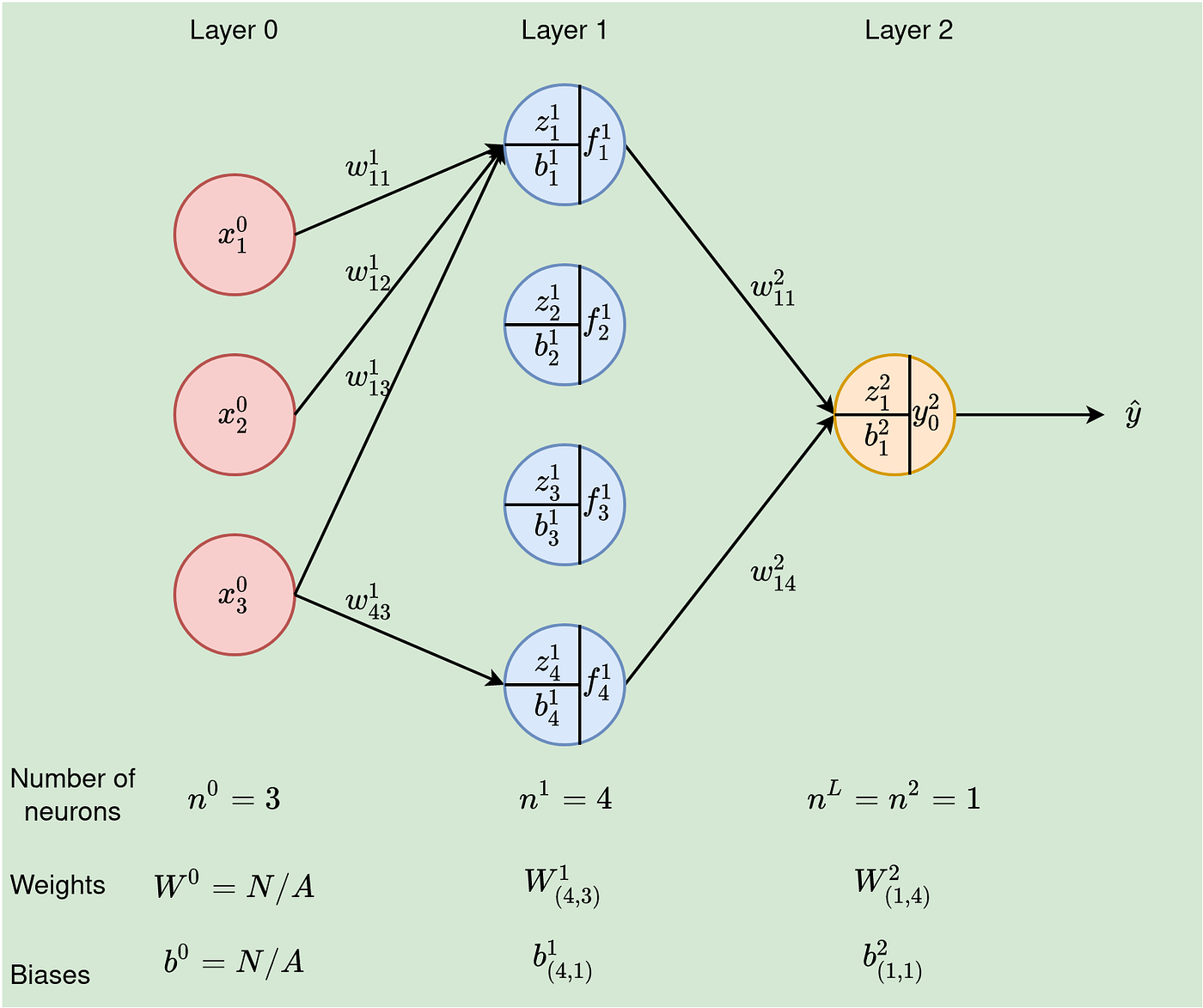
Here are the notations we will use:
- x⁰ᵢ — iᵗʰ input value. Value for feature i at the input layer (layer 0),
- nˡ — number of neurons in layer l. As shown in Figure 2, the first/input layer has three neurons, n⁰ =3, the second/hidden layer has 4 units, hence n¹=4, and lastly, for the output layer, n²=1. There are L layers in a network. In our case, L=2 (remember that we don’t count input as a layer because no calculations happen here),
- m — number of training examples. In our example here, m=1,
- wˡⱼᵢ — This weight comes from neuron i in layer l-1 to neuron j in the current layer l. Important: We will write wˡ to represent all the weights coming to any neurons in layer, l. This will, in most cases, be a matrix (we will come to it shortly),
- zˡⱼ — weighted input for jᵗʰ neuron in layer l,
- fˡⱼ = gˡ(zˡⱼ+bˡⱼ)— Output of unit j in layer l. This becomes the input to the units in the next layer, layer l+1. gˡ is the activation function at layer l, and,
- bˡⱼ — The bias on the jᵗʰ neuron of layer l.
To make the computation of neuron operations efficiently, we can use matrices and vectors for input, weights and biases for any given layer. We will now have the following matrices/vectors and operations:
- input as x,
- weights coming to layer l as matrix wˡ,
- biases in layer l as vector bˡ,
- zˡ = wˡ∙f^(l-1)— is the weighted input for all the neurons in layer, l. Medium.com has limitation in formatting. f is to power (l-1) for input from the previous layer.
- Dot product- For any two vectors a and b of equal-length, the dot product, a∙b is defined as:
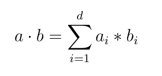
aᵢ* bᵢ is scalar multiplication between iᵗʰ element in vector a and iᵗʰ element in b.
- fˡ = gˡ(zˡ+bˡ) will be the output of layer l.
Matrix Multiplication
Two matrices can only be multiplied if they are compatible. Two matrices are said to be compatible for multiplication if and only if the number of columns for the first matrix is equal to the number of rows of the second matrix. Therefore, for A(m,n) and B(n,p), then A∙B is of order (m,p) (see Figure 2 below).
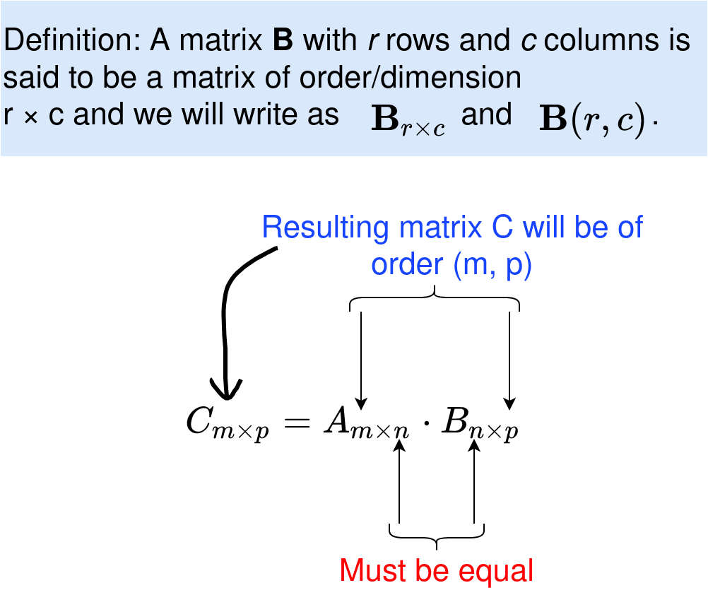
Important note: Matrix multiplication is NOT COMMUTATIVE, that is, A∙B is not equal to B∙A. Be sure you are multiplying them in the correct order.
Matrix Addition
Two matrices, A and B, can only be added if they are of the same dimension, say, A(m,n), then B must also be of order (m, n), and the result A+B is also of dimension (m, n).
Leveraging matrix operations in our network needs us to get the dimensions right for the input, weights, and biases.
To demonstrate the computations done in one neuron, let’s consider calculations in the first neuron of the hidden layer (note that weights are randomly generated and bias set to 0 at the start). In this section, we are basically assuming that we have a network of one neuron, that is, 3–1 NN.
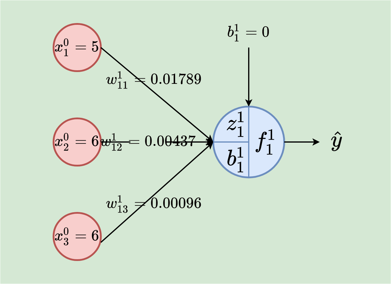
In this case, we have 3 input values 5, 6, and 6, and corresponding weights of 0.01789, 0.00437, and 0.00096. The neurons weigh the input by computing z¹₁₁, add the bias b¹₁₁ and lastly, apply an activation function (we will use the sigmoid function) on the result to get f¹₁₁ which makes the output.
Weighted input:
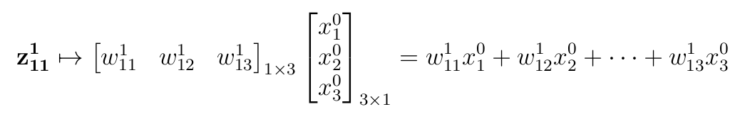
z¹₁₁ = (0.01789*5) + (0.00437*6) + (0.00096*6) = 0.12143
Adding bias then applying sigmoid activation function:
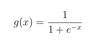
f¹₁₁ = g(z¹₁₁+b¹₁₁) = g(0.12143+0) = 1÷(1+e^(−0.12143)) = 0.530320253
This neuron outputs 0.5303.
Putting this into Python code
First of all, we need to generate weights randomly and set bias to zero.
Output:
Weights:  [[0.01789 0.00437 0.00096]]
Weights shape:  (1, 3)
Bias:  [[0.]]
Bias shape:  (1, 1)
Line 1–4: import numpy and set the precision for its output values to 5 decimal places. All computations performed by numpy after line 3 will be in 5 decimals place unless another precision level is set explicitly.
Line 5–8: In line 6 a randomization seed is set to 3 (it can be any number). Seeding ensures that the random numbers generated are predictable, that is, the random numbers generated are the same every time the code is run. Line 8 actually generates the random numbers using standard normal distribution. Why multiply it by 0.01? We want the number to be small (between 0 and 1). We will discuss this more in the next article
Line 11–14 just prints out parameter values and dimensions of matrices (see below for justification on the shapes of weights and bias matrices, very important!!!)
>>> Important Note on Dimensions<<<
We need to get dimensions of weights and biases matrices correctly. Given the number of neurons in each layer, the dimension for the matrices can be deduces as:
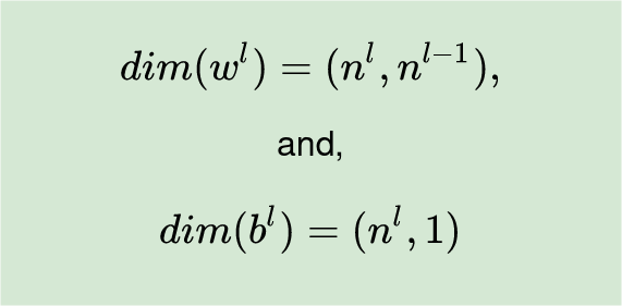
- The weights matrix for layer l (wˡ) will be of dimension (nˡ, n^(l-1)), that is, wˡ will have the number of rows equal to the number of neurons in the current layer, l, and the number of columns will be equal to the number of neurons in the previous layer, l-1.
- The bias matrix will have nˡ and 1 column. This is just a vector.
In our network, we have n⁰=3 input values and n¹ =1 neuron in the output, therefore, dim(w¹) = (n¹, n⁰) = (1, 3) and dim(b¹) = (n¹, 1) = (1,1). Hope this justifies the choice of shapes for the matrices of weights and biases.
Next is to multiply weights with input, add bias and apply sigmoid function.
Output:
input shape:  (3, 1)
f11:  [[0.12141]]
The output:  [[0.53032]]
Line 1–4 defines the input and prints the shape. Without reshaping the input, the result will be an array of shape (3,). Arrays of the nature (*, ), called rank 1 array, should be avoided because they will cause problems during matrix multiplication. The function reshape(-1, 1) tells numpy to dynamically set the number of rows and keep columns=1 for the array based on the number of values given. In our case, we have 3 input values, and therefore we have (3, 1) as the input shape.
Line 5 through 13 — multiply weights matrix with input matrix to get weighted input and add bias, then apply sigmoid activation to the result. When multiplying matrices in line 6, note the order — tt is the weights matrix multiplied by input and not the other way (remember the rules of matrix multiplication from the previous section?).
And the output is 0.5303. Note that it matches what we got previously.
Lets now put together all that
Output:
Weights:  [[0.01789 0.00437 0.00096]]
Weights shape:  (1, 3)
Bias:  [[0.]]
Bias shape:  (1, 1)
input values:  [[5]
[6]
[6]]
input shape:  (3, 1)
output [[0.53032]]
The class OneNeuronNeuralNetwork takes two arguments — weights and biases — which are initialized by magic/dunder function __init__.
The __init__ function is called every time an object is created from a class. The __init__ method lets the class initialize the object’s attributes and serves no other purpose — Source: Udacity.com
We use sigmoid_function as a static method because it is an ordinary function that does not have to receive the first argument “self”. We are just having it inside the class because it is relevant to be here otherwise it is not mandatory.
We have discussed about computations for a single neuron in the previous section. In the next article (I will post it by June 2, 2022), we will discuss how the entire network performs a single forward pass given some data.
Please sign up for medium membership at 5$ only per month to be able to read all my articles on medium and those of other writers.
You can also subscribe to get my article into your email inbox when I post.
Thank you for reading, unto the next!!!
Neural Network (NN) is a black box for so many people. We know that it works, but we don’t understand how it works. This article will demystify this belief by working on some examples to show how a neural network really works.
If some terms are not so clear in this article, I have already written two more articles to cover the real basics: article 1 and article 2.
In this first example, let us consider a simple case where we have a dataset of 3 features, a target variable and just one training example (in reality we can never have this kind of data, but, it will make a very good start).
Fact 1: The structure of the data influences the architecture chosen for modelling. In fact, the number of features on the dataset is equal to the number of the neurons in the input layer. In our example, shown in the Figure below, we have 3 features and therefore the input layer of the architecture must have 3 neurons.
The number of hidden layers affects the learning process, and therefore it is chosen based on the application. A network with several hidden layers is called Deep Neural Network (DNN). In this example, we are dealing with a Shallow NN, so to say. We have 3 neurons in the input/first layer, 4 neurons in the hidden layer, and 1 neuron in the output — a 3–4–1 Neural Network.
Let’s set some notations up front so that we can use them going forward without ambiguity. To do this, let us redraw the architecture above to show the parameters and variables used in the NN.
Here are the notations we will use:
- x⁰ᵢ — iᵗʰ input value. Value for feature i at the input layer (layer 0),
- nˡ — number of neurons in layer l. As shown in Figure 2, the first/input layer has three neurons, n⁰ =3, the second/hidden layer has 4 units, hence n¹=4, and lastly, for the output layer, n²=1. There are L layers in a network. In our case, L=2 (remember that we don’t count input as a layer because no calculations happen here),
- m — number of training examples. In our example here, m=1,
- wˡⱼᵢ — This weight comes from neuron i in layer l-1 to neuron j in the current layer l. Important: We will write wˡ to represent all the weights coming to any neurons in layer, l. This will, in most cases, be a matrix (we will come to it shortly),
- zˡⱼ — weighted input for jᵗʰ neuron in layer l,
- fˡⱼ = gˡ(zˡⱼ+bˡⱼ)— Output of unit j in layer l. This becomes the input to the units in the next layer, layer l+1. gˡ is the activation function at layer l, and,
- bˡⱼ — The bias on the jᵗʰ neuron of layer l.
To make the computation of neuron operations efficiently, we can use matrices and vectors for input, weights and biases for any given layer. We will now have the following matrices/vectors and operations:
- input as x,
- weights coming to layer l as matrix wˡ,
- biases in layer l as vector bˡ,
- zˡ = wˡ∙f^(l-1)— is the weighted input for all the neurons in layer, l. Medium.com has limitation in formatting. f is to power (l-1) for input from the previous layer.
- Dot product- For any two vectors a and b of equal-length, the dot product, a∙b is defined as:
aᵢ* bᵢ is scalar multiplication between iᵗʰ element in vector a and iᵗʰ element in b.
- fˡ = gˡ(zˡ+bˡ) will be the output of layer l.
Matrix Multiplication
Two matrices can only be multiplied if they are compatible. Two matrices are said to be compatible for multiplication if and only if the number of columns for the first matrix is equal to the number of rows of the second matrix. Therefore, for A(m,n) and B(n,p), then A∙B is of order (m,p) (see Figure 2 below).
Important note: Matrix multiplication is NOT COMMUTATIVE, that is, A∙B is not equal to B∙A. Be sure you are multiplying them in the correct order.
Matrix Addition
Two matrices, A and B, can only be added if they are of the same dimension, say, A(m,n), then B must also be of order (m, n), and the result A+B is also of dimension (m, n).
Leveraging matrix operations in our network needs us to get the dimensions right for the input, weights, and biases.
To demonstrate the computations done in one neuron, let’s consider calculations in the first neuron of the hidden layer (note that weights are randomly generated and bias set to 0 at the start). In this section, we are basically assuming that we have a network of one neuron, that is, 3–1 NN.
In this case, we have 3 input values 5, 6, and 6, and corresponding weights of 0.01789, 0.00437, and 0.00096. The neurons weigh the input by computing z¹₁₁, add the bias b¹₁₁ and lastly, apply an activation function (we will use the sigmoid function) on the result to get f¹₁₁ which makes the output.
Weighted input:
z¹₁₁ = (0.01789*5) + (0.00437*6) + (0.00096*6) = 0.12143
Adding bias then applying sigmoid activation function:
f¹₁₁ = g(z¹₁₁+b¹₁₁) = g(0.12143+0) = 1÷(1+e^(−0.12143)) = 0.530320253
This neuron outputs 0.5303.
Putting this into Python code
First of all, we need to generate weights randomly and set bias to zero.
Output:
Weights:  [[0.01789 0.00437 0.00096]]
Weights shape:  (1, 3)
Bias:  [[0.]]
Bias shape:  (1, 1)
Line 1–4: import numpy and set the precision for its output values to 5 decimal places. All computations performed by numpy after line 3 will be in 5 decimals place unless another precision level is set explicitly.
Line 5–8: In line 6 a randomization seed is set to 3 (it can be any number). Seeding ensures that the random numbers generated are predictable, that is, the random numbers generated are the same every time the code is run. Line 8 actually generates the random numbers using standard normal distribution. Why multiply it by 0.01? We want the number to be small (between 0 and 1). We will discuss this more in the next article
Line 11–14 just prints out parameter values and dimensions of matrices (see below for justification on the shapes of weights and bias matrices, very important!!!)
>>> Important Note on Dimensions<<<
We need to get dimensions of weights and biases matrices correctly. Given the number of neurons in each layer, the dimension for the matrices can be deduces as:
- The weights matrix for layer l (wˡ) will be of dimension (nˡ, n^(l-1)), that is, wˡ will have the number of rows equal to the number of neurons in the current layer, l, and the number of columns will be equal to the number of neurons in the previous layer, l-1.
- The bias matrix will have nˡ and 1 column. This is just a vector.
In our network, we have n⁰=3 input values and n¹ =1 neuron in the output, therefore, dim(w¹) = (n¹, n⁰) = (1, 3) and dim(b¹) = (n¹, 1) = (1,1). Hope this justifies the choice of shapes for the matrices of weights and biases.
Next is to multiply weights with input, add bias and apply sigmoid function.
Output:
input shape:  (3, 1)
f11:  [[0.12141]]
The output:  [[0.53032]]
Line 1–4 defines the input and prints the shape. Without reshaping the input, the result will be an array of shape (3,). Arrays of the nature (*, ), called rank 1 array, should be avoided because they will cause problems during matrix multiplication. The function reshape(-1, 1) tells numpy to dynamically set the number of rows and keep columns=1 for the array based on the number of values given. In our case, we have 3 input values, and therefore we have (3, 1) as the input shape.
Line 5 through 13 — multiply weights matrix with input matrix to get weighted input and add bias, then apply sigmoid activation to the result. When multiplying matrices in line 6, note the order — tt is the weights matrix multiplied by input and not the other way (remember the rules of matrix multiplication from the previous section?).
And the output is 0.5303. Note that it matches what we got previously.
Lets now put together all that
Output:
Weights:  [[0.01789 0.00437 0.00096]]
Weights shape:  (1, 3)
Bias:  [[0.]]
Bias shape:  (1, 1)
input values:  [[5]
[6]
[6]]
input shape:  (3, 1)
output [[0.53032]]
The class OneNeuronNeuralNetwork takes two arguments — weights and biases — which are initialized by magic/dunder function __init__.
The __init__ function is called every time an object is created from a class. The __init__ method lets the class initialize the object’s attributes and serves no other purpose — Source: Udacity.com
We use sigmoid_function as a static method because it is an ordinary function that does not have to receive the first argument “self”. We are just having it inside the class because it is relevant to be here otherwise it is not mandatory.
We have discussed about computations for a single neuron in the previous section. In the next article (I will post it by June 2, 2022), we will discuss how the entire network performs a single forward pass given some data.
Please sign up for medium membership at 5$ only per month to be able to read all my articles on medium and those of other writers.
You can also subscribe to get my article into your email inbox when I post.
Thank you for reading, unto the next!!!
Denial of responsibility! Techno Blender is an automatic aggregator of the all world’s media. In each content, the hyperlink to the primary source is specified. All trademarks belong to their rightful owners, all materials to their authors. If you are the owner of the content and do not want us to publish your materials, please contact us by email – [email protected]. The content will be deleted within 24 hours.