
IVFPQ + HNSW for Billion-scale Similarity Search | by Peggy Chang | Towards Data Science
The best indexing approach for billion-sized vector datasets
We learned about IVFPQ in the previous article, where the inverted file index (IVF) is combined with product quantization (PQ) to create an effective method for large-scale similarity search.
In this article, we will learn about HNSW and how it can be used together with IVFPQ to form the best indexing approach for billion-scale similarity search.
We will first introduce NSW and skip list, the two important foundations that HNSW is built upon. We will also go through the implementation of HNSW using Faiss, the effect of different parameter settings, as well as how the different variations of HNSW indexes compare over search quality, speed, and memory usage.
1. Introduction
2. Navigable Small World (NSW)
∘ (A) NSW — Construction
∘ (B) NSW — Search
3. Skip List
4. Hierarchical Navigable Small World (HNSW)
∘ (A) HNSW — Construction
∘ Insertion Process
∘ Heuristic Selection
∘ (B) HNSW — Search
5. Implementation with Faiss: IndexHNSWFlat
∘ Effect of M, efConstruction, and efSearch
6. Implementation with Faiss: IndexIVFPQ + HNSW
7. Comparison of HNSW indexes (with/without IVF and/or PQ)
8. Summary
A graph consists of vertices and edges. An edge is a line that connects two vertices together. Let’s call connected vertices friends.
In the world of vectors, similar vectors are often located close to one another. Thus if vectors are represented as vertices on a graph, logically, vertices that are close together (i.e. vectors with high similarity) should be connected as friends. Even if they’re not connected as friends, they should be reachable by each other easily by traversing just one or two other vertices.
For a graph to be navigable, every vertex must have friends. Else there is no way to reach the vertex. Having friends is great, but having too many friends can be very costly for a graph. Just think of the memory and storage required to keep those connections and the number of computations needed to compare distances during search time.
Typically, we do not want a graph that looks like the following.
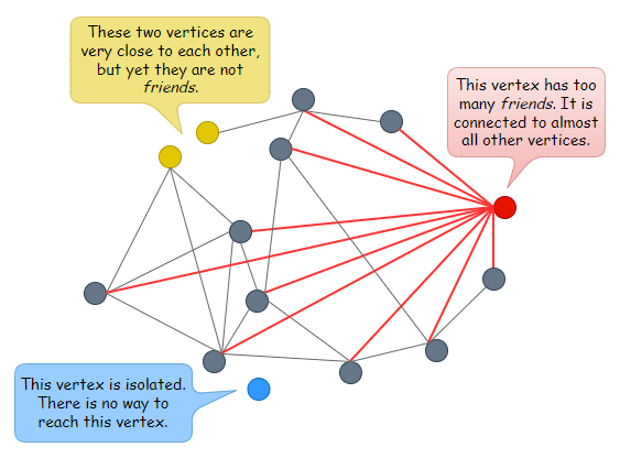
What we want is a navigable graph that has the properties of a small-world network, one where each vertex has only a small number of connections, and one where the average hop count between two randomly chosen vertices is low.
Conceptually, using a Delaunay graph (or Delaunay triangulation) for the approximate nearest neighbor search seemed ideal since vertices that are close to each other are friends, and isolated vertex does not exist.

However, constructing a Delaunay graph is not easy and straightforward, and the search efficiency is just sub-optimal. For example, if two vertices A and B are located very far apart, we need to pass through a large number of friend connections starting from A to reach B, and vice versa.
Therefore, instead of building an exact Delaunay graph, NSW uses a simpler approach to build an approximation of the Delaunay graph.
(A) NSW — Construction
The NSW graph is built by inserting vertices one after another in random order (i.e. the vectors are first shuffled).
When a new vertex is inserted, it will be connected to
Mexisting vertices that are closest to it.
In the illustration below, M is set to 3. We start by inserting A. At this point, there is no other vertex in the graph. Next, we insert B. Since there is only A in the graph, we connect B to A. Then we insert C. Now there is only A and B in the graph, so we connect C to A and B. Following that, we insert D. Similarly, since there are only A, B, and C in the graph, we connect D to A, B, and C.
Now when we insert E, there are four other vertices in the graph, i.e. A, B, C, and D. Since M is set to 3, we connect E only to the three nearest vertices, i.e. B, C, and D.
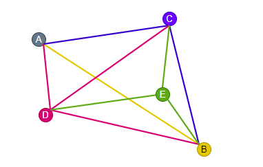
M=3If we continue to insert vertices and build the graph in this manner, we could come out with an NSW graph that looks like the following.

As more and more vertices are inserted, it can be observed that some of the connections built during the early stages have become long-range links. For example, look at the links ‘A — B’ and ‘C — D’ in the graph above.
(B) NSW — Search
The search on an NSW graph follows a simple greedy search method.
Only local information is used on each step, and no prior global knowledge of dimensionality or distribution of the data is required. This is the beauty of NSW, and a search can be initiated from any vertex.
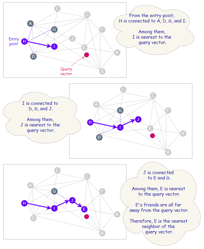
The entry point for the search can be randomly selected. From the current point, the algorithm would try to find a friend that is nearest to the query vector and move towards that vertex.
As depicted below, the step is repeated until it can no longer find any friend that is closer to the query vector than itself.
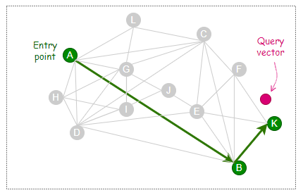
The following illustration shows how the long-range links created during the early phase of the construction can benefit some search cases. In this example, the entry point, A, and query vector are located at opposite ends of the graph. Thanks to the long-range link ‘A — B’, the search process takes only two hops (A→B→K) to reach the nearest neighbor of the query vector.
Search quality for NSW can be improved by performing multiple searches with random entry points.
The skip list is a data structure invented by W. Pugh [3], which is built based on linked list with sorted elements.
Below is an example of a linked list where the elements are already in sorted order. A node on a linked list contains the element’s value and a pointer to the next element.
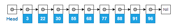
Skip list is made up of multiple layers of linked list, where the original linked list is at the bottom (Level 0). The upper levels contain the same elements found on Level 0, but only a subset of them. The number of elements gets lesser as the level number goes up.
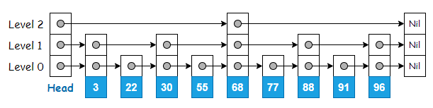
Upper levels of the skip list serve as expressways since some elements are skipped during traversal.
This makes searching for an element fast on a skip list. The search starts from the top-most level, traversing the nodes and going down the level only if the current pointer points to the next element where its value is greater than what is being searched for.
For example, searching for ‘91’ involves traversing only 3 nodes, as opposed to 8 nodes if the search is to be done on the original linked list.

HNSW is a new evolution of NSW, where the hierarchies constitute an elegant refinement and are inspired by the layering structure from skip list.
The hierarchical composition in HNSW segregates links with different length scales into different layers. Long-range links can be found on the upper levels, while short-range links are at the bottom.
Long-range links play an important role in reducing the time and effort spent to reach the vicinity of the nearest neighbor that one is looking for.

(A) HNSW — Construction
The construction of HNSW is very similar to NSW, in which the graph structure is also incrementally built by inserting vertices one after another.
However, unlike NSW, the vertices do not need to be shuffled before insertion. This is because the stochastic effect in HNSW is accomplished by level randomization. How does this work?
Well, during graph construction, each vertex is randomly assigned an integer, ℓ, indicating the maximum layer in which the vertex is present. For instance, if a vertex is assigned with ℓ=3, then we can find the vertex present at Level 2, Level 1, and Level 0.
“The maximum layer in which an element is present is selected randomly with an exponentially decaying probability distribution” — Y. Malkov and D. Yashunin
This makes ℓ=1 the most likely assignment that a vertex will receive, and getting larger ℓ values happen with exponentially low probability.
Hence, the majority of vertices are always seen to be present at Level 0. As the level number goes up, the number of vertices present at those levels decreases significantly. To get a sense of what the distribution looks like for ℓ, take a look at the sample below from a random dataset of 500,000 vectors.

Insertion Process
During the insertion process, on each level, the algorithm greedily explores the neighborhood of vertices and maintains a dynamic list of currently found nearest neighbors of the newly inserted vertex.
For the first phase of the insertion process that starts from the top level, the size of this dynamic list is set to 1. The found closest vertex is then used as an entry point to the next layer beneath, and the search continues.
Once the level that is lower than ℓ is reached, this marks the second phase of the insertion process. From this point onwards, the size of the dynamic list follows the value set by a parameter called efConstruction. Besides acting as entry points to the next layer beneath (if any), the currently found nearest neighbors are also candidate friends, out of which M of them would be selected to make connections with the newly inserted vertex on the current level.
The insertion process ends when connections of the newly inserted vertex are established at Level 0.
According to the paper [2], “the dynamic list is updated at each step by evaluating the neighborhood of the closest previously non-evaluated element in the list until the neighborhood of every element from the list is evaluated”.
Thus
efConstruction(that sets the size of the dynamic candidate list) can be defined as the parameter that controls the number of candidate neighbors to explore. It signifies the depth of exploration during construction time.
Heuristic Selection
Earlier, we learned that for NSW, the M existing vertices that are closest to the new vertex would be selected to make connections. This is a simple approach of selecting and connecting only to the closest vertices. For HNSW, using the heuristic to establish connections is one step ahead in elevating performance.
Heuristic selection not only takes into account the shortest distance between vertices but also the connectivity of different regions on the graph.
Consider the example below. It is very obvious that the two clusters on the right are not directly connected. In order to go from A to Y, one has to traverse a long route, passing through another cluster on the left.

With M=2, when we insert a new vertex N at the position shown below, we get 4 candidate friends, A, B, X, and Y, out of which 2 would be chosen to connect with N.
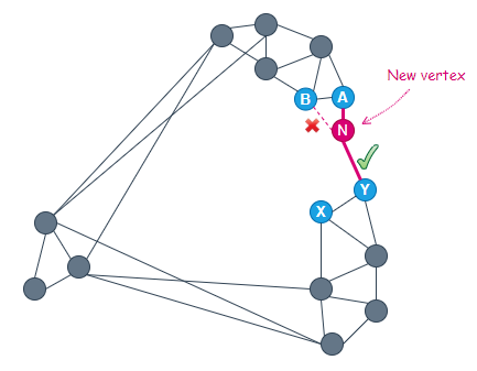
Of the 4 candidates, A is closest to the new vertex. Therefore, A is selected to connect to N.
The next closest vertex to N is B. However, because the distance ‘B — A’ is smaller than that of ‘B — N’, vertex B is ignored and the next closest vertex, Y, is considered.
At this point, the heuristic chooses to connect N to Y since the distance ‘Y — A’ is greater than that of ‘Y — N’. By doing so, we are now able to have a direct connection between the two clusters on the right.
The heuristic enhances the diversity of a vertex’s neighborhood and leads to better search efficiency for the case of highly clustered data.
During construction, besides establishing M connections for every new vertex, HNSW also keeps an eye on the total number of connections that each vertex is having at any point in time. In order to maintain the small world navigability, the maximum number of connections per vertex is usually capped at 2*M for Level 0, and M for all other levels.
For query vector search, the speed is influenced by M, efConstruction, and efSearch. The search generally gets slower when the values of these parameters increase.

The same parameters also affect the search quality. Higher recalls can be obtained by having larger values for M, efConstruction, or efSearch.
Note that setting efConstruction with a value that is too small is not useful in getting a reasonable performance. Raising the value of M or efSearch under this circumstance does not help. To achieve satisfactory results, a feasible value for efConstruction is absolutely necessary.
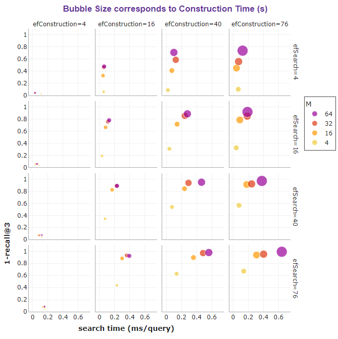
For example, in our case, efConstruction=40 together with M=32 and efSearch=16 is able to reach an impressive recall of 0.85 at a fast search speed of 0.24 ms per query. This means the true nearest neighbor is returned within the first 3 results of each query 85% of the time.
If we do not mind a slower search, increasing efSearch to 76 can even boost recall to a near-perfect score of 0.97!
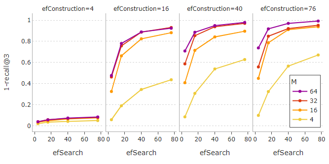
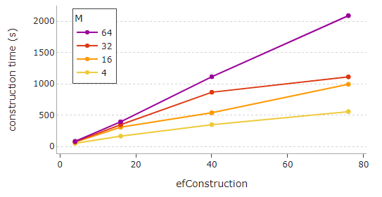
It can be seen that the recall slowly starts to plateau after a certain point for high values of M, efSearch, and efConstruction. Also, be mindful that setting high values for M and efConstruction can cause a notably longer construction time, as portrayed below.
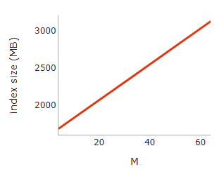
Lastly, the index size of HNSW, which is indicative of memory usage, grows linearly with M.
The bubble charts below summarize the effect of M, efConstruction, and efSearch on the search speed and accuracy of HNSW, as well as on the index size and construction time.

If memory is not a concern, HNSW is a great choice for providing fast and superb-quality searches.
Awesome! We’ve learned how to implement HNSW with Faiss. But how do we use HNSW with IVFPQ?
In Faiss, IVFPQ is implemented with IndexIVFPQ.
The
IndexHNSWFlatwe saw earlier now works as the coarse quantizer forIndexIVFPQ.The coarse quantizer is responsible for finding the partition centroids that are nearest to the query vector so that vector search only needs to be performed on those partitions.
The codes below show how to create a IndexIVFPQ with IndexHNSWFlat as the coarse quantizer.
Note that IndexIVFPQ needs to be trained with k-means clustering before database vectors are added. To do this, the train method is used. Once the index is created, the value of nprobe can be set to specify the number of partitions to search.
In Faiss, an index can also be created using the
index_factoryfunction instead of the class constructor. This alternative is useful, especially for building complex composite indexes that could possibly include preprocessing steps such as PCA, or other kinds of vector transformation and refinement.With the
index_factory, several lines of codes can be simplified to only one line by specifying the dimension of vectors (e.g. 128) and the factory string (e.g. “IVF10000_HNSW32,PQ16”) as inputs to the function.
index = faiss.index_factory(128, "IVF10000_HNSW32,PQ16")
The line above uses the
index_factoryto creates an index for 128-dimensional vectors. It is an inverted file index with 10,000 partitions and uses Product Quantization with 16 segments of 8 bits each (if the number of bits is not specified, 8 bits is the default). The coarse quantizer is a graph-based HNSW index with 32 connections to be made for every new vertex.
In this section, we will look at the different variations of HNSW indexes and how they compare in terms of search accuracy, speed, and memory usage. They are:
- IVFPQ+HNSW
- IVF+HNSW
- HNSW
- HNSW+PQ
The Faiss index_factory is used to create these four types of indexes with the following factory strings:
IVF65536_HNSW32,PQ32: This is essentially IVFPQ+HNSW. It is an inverted file index with 65,536 partitions that uses Product Quantization with 32 segments of 8 bits each. The coarse quantizer is a graph-based HNSW index with
M=32.IVF65536_HNSW32,Flat: This is essentially IVF+HNSW. It is an inverted file index with 65,536 partitions. The coarse quantizer is a graph-based HNSW index with
M=32.HNSW32,Flat: This is essentially just HNSW, a graph-based index with
M=32.HNSW32_PQ32: This is essentially HNSW+PQ. It is a graph-based HNSW index with
M=32, and uses Product Quantization with 32 segments of 8 bits each.
Same as before, 3 million 128-dimensional vectors are added to these indexes, and search is performed using 1,000 query vectors. As for efConstruction and efSearch, the default values from Faiss are used.
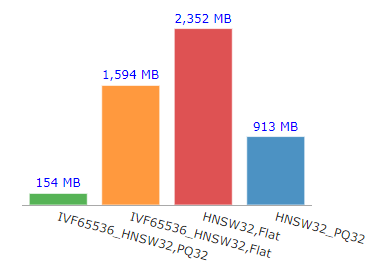
Out of the four types of indexes, IVFPQ+HNSW appeared as the champion in terms of index size or memory usage. With just 154 MB in size, it is 15 times more memory efficient than HNSW alone.
For IVF-based indexes, increasing nprobe (the number of partitions to search) results in a longer search time but better recall performance.
Depending on the value of nprobe used, IVF-based indexes can perform better or poorer than HNSW or HNSW+PQ.
From the graphs below, we can get a sense of the relative performance of the indexes when nprobe=128 is used for IVF-based indexes.

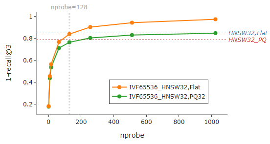
Selecting an appropriate
nprobeis key to balancing the trade-offs between search speed and accuracy.
The recall performance versus search time taken by the four types of indexes, as well as their respective sizes in MB, are shown in this table.
nprobe used is 128.The results can be visualized from the charts below. On the bar chart, we can witness vast differences with respect to search speed from the four types of indexes, compared to the more subtle differences in recall performance.

The bubble chart below provides a good visual overview of search time versus recall performance. The size of the bubble corresponds to the size of the index, which is indicative of memory usage.

In terms of search speed, it can be observed that IVF-based indexes (green and orange bubbles) are leading the race. They are incredibly fast due to the non-exhaustive nature of the search, as the search is only performed on a small subset of partitions.
In terms of accuracy, HNSW (red bubble) comes first, while PQ indexes (green and blue bubbles) are lagging behind. PQ indexes are indexes with Product Quantization. They are anticipated to have lower accuracy due to the lossy compression that they make. However, their weakness is highly compensated by huge savings in memory.
Clearly, IVFPQ+HNSW (green bubble) is the winner both in terms of search speed and memory efficiency. It has the smallest memory footprint (ooh, look at how tiny the green bubble is), and by using nprobe=128, it managed to achieve the fastest average search time of 0.03 ms per query, all with a good recall of 0.77.
What if a higher recall is desired? As illustrated below, increasing nprobe does the trick, but at the cost of longer search time. Remember, selecting an appropriate nprobe is fundamental for achieving sensible and realistic outcomes amid balancing the trade-offs.
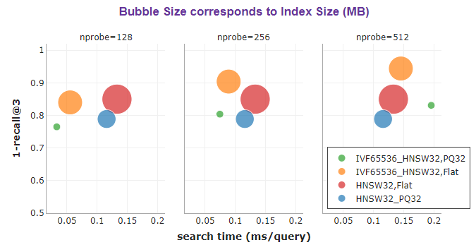
nprobe for IVF-based indexes. The green and orange bubbles move towards the top and right when nprobe increases.IVFPQ together with HNSW as the coarse quantizer delivers an extremely memory-efficient and impeccable fast search that is of good accuracy for large-scale approximate nearest neighbor search.
It is not surprising that with a good balance of speed, memory usage, and accuracy, IVFPQ+HNSW makes the best indexing approach for billion-scale similarity search.
[1] Y. Malkov, A. Ponomarenko, A. Logvinov and V. Krylov, Approximate nearest neighbor algorithm based on navigable small world graphs (2013)
[2] Y. Malkov and D. Yashunin, Efficient and robust approximate nearest neighbor search using Hierarchical Navigable Small World graphs (2018)
[3] W. Pugh, Skip Lists: A Probabilistic Alternative to Balanced Trees (1990), Communications of the ACM, vol. 33, no.6, pp. 668–676
[4] J. Briggs, Hierarchical Navigable Small Worlds (HNSW)
[5] Y. Matsui, Billion-scale Approximate Nearest Neighbor Search (2020)
[6] Faiss Wiki
[7] J. Arguello, Evaluation Metrics
Before You Go...Thank you for reading this post, and I hope you’ve enjoyed learning the best indexing approach for billion-scale similarity search.If you like my post, don’t forget to hit Follow and Subscribe to get notified via email when I publish.Optionally, you may also sign up for a Medium membership to get full access to every story on Medium.📑 Visit this GitHub repo for all codes and notebooks that I shared in my posts.© 2022 All rights reserved.
Interested to read my other data science articles? Check out the following:
Series on Mastering Dynamic Programming


The best indexing approach for billion-sized vector datasets
We learned about IVFPQ in the previous article, where the inverted file index (IVF) is combined with product quantization (PQ) to create an effective method for large-scale similarity search.
In this article, we will learn about HNSW and how it can be used together with IVFPQ to form the best indexing approach for billion-scale similarity search.
We will first introduce NSW and skip list, the two important foundations that HNSW is built upon. We will also go through the implementation of HNSW using Faiss, the effect of different parameter settings, as well as how the different variations of HNSW indexes compare over search quality, speed, and memory usage.
1. Introduction
2. Navigable Small World (NSW)
∘ (A) NSW — Construction
∘ (B) NSW — Search
3. Skip List
4. Hierarchical Navigable Small World (HNSW)
∘ (A) HNSW — Construction
∘ Insertion Process
∘ Heuristic Selection
∘ (B) HNSW — Search
5. Implementation with Faiss: IndexHNSWFlat
∘ Effect of M, efConstruction, and efSearch
6. Implementation with Faiss: IndexIVFPQ + HNSW
7. Comparison of HNSW indexes (with/without IVF and/or PQ)
8. Summary
A graph consists of vertices and edges. An edge is a line that connects two vertices together. Let’s call connected vertices friends.
In the world of vectors, similar vectors are often located close to one another. Thus if vectors are represented as vertices on a graph, logically, vertices that are close together (i.e. vectors with high similarity) should be connected as friends. Even if they’re not connected as friends, they should be reachable by each other easily by traversing just one or two other vertices.
For a graph to be navigable, every vertex must have friends. Else there is no way to reach the vertex. Having friends is great, but having too many friends can be very costly for a graph. Just think of the memory and storage required to keep those connections and the number of computations needed to compare distances during search time.
Typically, we do not want a graph that looks like the following.
What we want is a navigable graph that has the properties of a small-world network, one where each vertex has only a small number of connections, and one where the average hop count between two randomly chosen vertices is low.
Conceptually, using a Delaunay graph (or Delaunay triangulation) for the approximate nearest neighbor search seemed ideal since vertices that are close to each other are friends, and isolated vertex does not exist.
However, constructing a Delaunay graph is not easy and straightforward, and the search efficiency is just sub-optimal. For example, if two vertices A and B are located very far apart, we need to pass through a large number of friend connections starting from A to reach B, and vice versa.
Therefore, instead of building an exact Delaunay graph, NSW uses a simpler approach to build an approximation of the Delaunay graph.
(A) NSW — Construction
The NSW graph is built by inserting vertices one after another in random order (i.e. the vectors are first shuffled).
When a new vertex is inserted, it will be connected to
Mexisting vertices that are closest to it.
In the illustration below, M is set to 3. We start by inserting A. At this point, there is no other vertex in the graph. Next, we insert B. Since there is only A in the graph, we connect B to A. Then we insert C. Now there is only A and B in the graph, so we connect C to A and B. Following that, we insert D. Similarly, since there are only A, B, and C in the graph, we connect D to A, B, and C.
Now when we insert E, there are four other vertices in the graph, i.e. A, B, C, and D. Since M is set to 3, we connect E only to the three nearest vertices, i.e. B, C, and D.
M=3If we continue to insert vertices and build the graph in this manner, we could come out with an NSW graph that looks like the following.
As more and more vertices are inserted, it can be observed that some of the connections built during the early stages have become long-range links. For example, look at the links ‘A — B’ and ‘C — D’ in the graph above.
(B) NSW — Search
The search on an NSW graph follows a simple greedy search method.
Only local information is used on each step, and no prior global knowledge of dimensionality or distribution of the data is required. This is the beauty of NSW, and a search can be initiated from any vertex.
The entry point for the search can be randomly selected. From the current point, the algorithm would try to find a friend that is nearest to the query vector and move towards that vertex.
As depicted below, the step is repeated until it can no longer find any friend that is closer to the query vector than itself.
The following illustration shows how the long-range links created during the early phase of the construction can benefit some search cases. In this example, the entry point, A, and query vector are located at opposite ends of the graph. Thanks to the long-range link ‘A — B’, the search process takes only two hops (A→B→K) to reach the nearest neighbor of the query vector.
Search quality for NSW can be improved by performing multiple searches with random entry points.
The skip list is a data structure invented by W. Pugh [3], which is built based on linked list with sorted elements.
Below is an example of a linked list where the elements are already in sorted order. A node on a linked list contains the element’s value and a pointer to the next element.
Skip list is made up of multiple layers of linked list, where the original linked list is at the bottom (Level 0). The upper levels contain the same elements found on Level 0, but only a subset of them. The number of elements gets lesser as the level number goes up.
Upper levels of the skip list serve as expressways since some elements are skipped during traversal.
This makes searching for an element fast on a skip list. The search starts from the top-most level, traversing the nodes and going down the level only if the current pointer points to the next element where its value is greater than what is being searched for.
For example, searching for ‘91’ involves traversing only 3 nodes, as opposed to 8 nodes if the search is to be done on the original linked list.
HNSW is a new evolution of NSW, where the hierarchies constitute an elegant refinement and are inspired by the layering structure from skip list.
The hierarchical composition in HNSW segregates links with different length scales into different layers. Long-range links can be found on the upper levels, while short-range links are at the bottom.
Long-range links play an important role in reducing the time and effort spent to reach the vicinity of the nearest neighbor that one is looking for.
(A) HNSW — Construction
The construction of HNSW is very similar to NSW, in which the graph structure is also incrementally built by inserting vertices one after another.
However, unlike NSW, the vertices do not need to be shuffled before insertion. This is because the stochastic effect in HNSW is accomplished by level randomization. How does this work?
Well, during graph construction, each vertex is randomly assigned an integer, ℓ, indicating the maximum layer in which the vertex is present. For instance, if a vertex is assigned with ℓ=3, then we can find the vertex present at Level 2, Level 1, and Level 0.
“The maximum layer in which an element is present is selected randomly with an exponentially decaying probability distribution” — Y. Malkov and D. Yashunin
This makes ℓ=1 the most likely assignment that a vertex will receive, and getting larger ℓ values happen with exponentially low probability.
Hence, the majority of vertices are always seen to be present at Level 0. As the level number goes up, the number of vertices present at those levels decreases significantly. To get a sense of what the distribution looks like for ℓ, take a look at the sample below from a random dataset of 500,000 vectors.
Insertion Process
During the insertion process, on each level, the algorithm greedily explores the neighborhood of vertices and maintains a dynamic list of currently found nearest neighbors of the newly inserted vertex.
For the first phase of the insertion process that starts from the top level, the size of this dynamic list is set to 1. The found closest vertex is then used as an entry point to the next layer beneath, and the search continues.
Once the level that is lower than ℓ is reached, this marks the second phase of the insertion process. From this point onwards, the size of the dynamic list follows the value set by a parameter called efConstruction. Besides acting as entry points to the next layer beneath (if any), the currently found nearest neighbors are also candidate friends, out of which M of them would be selected to make connections with the newly inserted vertex on the current level.
The insertion process ends when connections of the newly inserted vertex are established at Level 0.
According to the paper [2], “the dynamic list is updated at each step by evaluating the neighborhood of the closest previously non-evaluated element in the list until the neighborhood of every element from the list is evaluated”.
Thus
efConstruction(that sets the size of the dynamic candidate list) can be defined as the parameter that controls the number of candidate neighbors to explore. It signifies the depth of exploration during construction time.
Heuristic Selection
Earlier, we learned that for NSW, the M existing vertices that are closest to the new vertex would be selected to make connections. This is a simple approach of selecting and connecting only to the closest vertices. For HNSW, using the heuristic to establish connections is one step ahead in elevating performance.
Heuristic selection not only takes into account the shortest distance between vertices but also the connectivity of different regions on the graph.
Consider the example below. It is very obvious that the two clusters on the right are not directly connected. In order to go from A to Y, one has to traverse a long route, passing through another cluster on the left.
With M=2, when we insert a new vertex N at the position shown below, we get 4 candidate friends, A, B, X, and Y, out of which 2 would be chosen to connect with N.
Of the 4 candidates, A is closest to the new vertex. Therefore, A is selected to connect to N.
The next closest vertex to N is B. However, because the distance ‘B — A’ is smaller than that of ‘B — N’, vertex B is ignored and the next closest vertex, Y, is considered.
At this point, the heuristic chooses to connect N to Y since the distance ‘Y — A’ is greater than that of ‘Y — N’. By doing so, we are now able to have a direct connection between the two clusters on the right.
The heuristic enhances the diversity of a vertex’s neighborhood and leads to better search efficiency for the case of highly clustered data.
During construction, besides establishing M connections for every new vertex, HNSW also keeps an eye on the total number of connections that each vertex is having at any point in time. In order to maintain the small world navigability, the maximum number of connections per vertex is usually capped at 2*M for Level 0, and M for all other levels.
For query vector search, the speed is influenced by M, efConstruction, and efSearch. The search generally gets slower when the values of these parameters increase.
The same parameters also affect the search quality. Higher recalls can be obtained by having larger values for M, efConstruction, or efSearch.
Note that setting efConstruction with a value that is too small is not useful in getting a reasonable performance. Raising the value of M or efSearch under this circumstance does not help. To achieve satisfactory results, a feasible value for efConstruction is absolutely necessary.
For example, in our case, efConstruction=40 together with M=32 and efSearch=16 is able to reach an impressive recall of 0.85 at a fast search speed of 0.24 ms per query. This means the true nearest neighbor is returned within the first 3 results of each query 85% of the time.
If we do not mind a slower search, increasing efSearch to 76 can even boost recall to a near-perfect score of 0.97!
It can be seen that the recall slowly starts to plateau after a certain point for high values of M, efSearch, and efConstruction. Also, be mindful that setting high values for M and efConstruction can cause a notably longer construction time, as portrayed below.
Lastly, the index size of HNSW, which is indicative of memory usage, grows linearly with M.
The bubble charts below summarize the effect of M, efConstruction, and efSearch on the search speed and accuracy of HNSW, as well as on the index size and construction time.
If memory is not a concern, HNSW is a great choice for providing fast and superb-quality searches.
Awesome! We’ve learned how to implement HNSW with Faiss. But how do we use HNSW with IVFPQ?
In Faiss, IVFPQ is implemented with IndexIVFPQ.
The
IndexHNSWFlatwe saw earlier now works as the coarse quantizer forIndexIVFPQ.The coarse quantizer is responsible for finding the partition centroids that are nearest to the query vector so that vector search only needs to be performed on those partitions.
The codes below show how to create a IndexIVFPQ with IndexHNSWFlat as the coarse quantizer.
Note that IndexIVFPQ needs to be trained with k-means clustering before database vectors are added. To do this, the train method is used. Once the index is created, the value of nprobe can be set to specify the number of partitions to search.
In Faiss, an index can also be created using the
index_factoryfunction instead of the class constructor. This alternative is useful, especially for building complex composite indexes that could possibly include preprocessing steps such as PCA, or other kinds of vector transformation and refinement.With the
index_factory, several lines of codes can be simplified to only one line by specifying the dimension of vectors (e.g. 128) and the factory string (e.g. “IVF10000_HNSW32,PQ16”) as inputs to the function.
index = faiss.index_factory(128, "IVF10000_HNSW32,PQ16")
The line above uses the
index_factoryto creates an index for 128-dimensional vectors. It is an inverted file index with 10,000 partitions and uses Product Quantization with 16 segments of 8 bits each (if the number of bits is not specified, 8 bits is the default). The coarse quantizer is a graph-based HNSW index with 32 connections to be made for every new vertex.
In this section, we will look at the different variations of HNSW indexes and how they compare in terms of search accuracy, speed, and memory usage. They are:
- IVFPQ+HNSW
- IVF+HNSW
- HNSW
- HNSW+PQ
The Faiss index_factory is used to create these four types of indexes with the following factory strings:
IVF65536_HNSW32,PQ32: This is essentially IVFPQ+HNSW. It is an inverted file index with 65,536 partitions that uses Product Quantization with 32 segments of 8 bits each. The coarse quantizer is a graph-based HNSW index with
M=32.IVF65536_HNSW32,Flat: This is essentially IVF+HNSW. It is an inverted file index with 65,536 partitions. The coarse quantizer is a graph-based HNSW index with
M=32.HNSW32,Flat: This is essentially just HNSW, a graph-based index with
M=32.HNSW32_PQ32: This is essentially HNSW+PQ. It is a graph-based HNSW index with
M=32, and uses Product Quantization with 32 segments of 8 bits each.
Same as before, 3 million 128-dimensional vectors are added to these indexes, and search is performed using 1,000 query vectors. As for efConstruction and efSearch, the default values from Faiss are used.
Out of the four types of indexes, IVFPQ+HNSW appeared as the champion in terms of index size or memory usage. With just 154 MB in size, it is 15 times more memory efficient than HNSW alone.
For IVF-based indexes, increasing nprobe (the number of partitions to search) results in a longer search time but better recall performance.
Depending on the value of nprobe used, IVF-based indexes can perform better or poorer than HNSW or HNSW+PQ.
From the graphs below, we can get a sense of the relative performance of the indexes when nprobe=128 is used for IVF-based indexes.
Selecting an appropriate
nprobeis key to balancing the trade-offs between search speed and accuracy.
The recall performance versus search time taken by the four types of indexes, as well as their respective sizes in MB, are shown in this table.
nprobe used is 128.The results can be visualized from the charts below. On the bar chart, we can witness vast differences with respect to search speed from the four types of indexes, compared to the more subtle differences in recall performance.
The bubble chart below provides a good visual overview of search time versus recall performance. The size of the bubble corresponds to the size of the index, which is indicative of memory usage.
In terms of search speed, it can be observed that IVF-based indexes (green and orange bubbles) are leading the race. They are incredibly fast due to the non-exhaustive nature of the search, as the search is only performed on a small subset of partitions.
In terms of accuracy, HNSW (red bubble) comes first, while PQ indexes (green and blue bubbles) are lagging behind. PQ indexes are indexes with Product Quantization. They are anticipated to have lower accuracy due to the lossy compression that they make. However, their weakness is highly compensated by huge savings in memory.
Clearly, IVFPQ+HNSW (green bubble) is the winner both in terms of search speed and memory efficiency. It has the smallest memory footprint (ooh, look at how tiny the green bubble is), and by using nprobe=128, it managed to achieve the fastest average search time of 0.03 ms per query, all with a good recall of 0.77.
What if a higher recall is desired? As illustrated below, increasing nprobe does the trick, but at the cost of longer search time. Remember, selecting an appropriate nprobe is fundamental for achieving sensible and realistic outcomes amid balancing the trade-offs.
nprobe for IVF-based indexes. The green and orange bubbles move towards the top and right when nprobe increases.IVFPQ together with HNSW as the coarse quantizer delivers an extremely memory-efficient and impeccable fast search that is of good accuracy for large-scale approximate nearest neighbor search.
It is not surprising that with a good balance of speed, memory usage, and accuracy, IVFPQ+HNSW makes the best indexing approach for billion-scale similarity search.
[1] Y. Malkov, A. Ponomarenko, A. Logvinov and V. Krylov, Approximate nearest neighbor algorithm based on navigable small world graphs (2013)
[2] Y. Malkov and D. Yashunin, Efficient and robust approximate nearest neighbor search using Hierarchical Navigable Small World graphs (2018)
[3] W. Pugh, Skip Lists: A Probabilistic Alternative to Balanced Trees (1990), Communications of the ACM, vol. 33, no.6, pp. 668–676
[4] J. Briggs, Hierarchical Navigable Small Worlds (HNSW)
[5] Y. Matsui, Billion-scale Approximate Nearest Neighbor Search (2020)
[6] Faiss Wiki
[7] J. Arguello, Evaluation Metrics
Before You Go...Thank you for reading this post, and I hope you’ve enjoyed learning the best indexing approach for billion-scale similarity search.If you like my post, don’t forget to hit Follow and Subscribe to get notified via email when I publish.Optionally, you may also sign up for a Medium membership to get full access to every story on Medium.📑 Visit this GitHub repo for all codes and notebooks that I shared in my posts.© 2022 All rights reserved.
Interested to read my other data science articles? Check out the following:
Series on Mastering Dynamic Programming
Denial of responsibility! Techno Blender is an automatic aggregator of the all world’s media. In each content, the hyperlink to the primary source is specified. All trademarks belong to their rightful owners, all materials to their authors. If you are the owner of the content and do not want us to publish your materials, please contact us by email – [email protected]. The content will be deleted within 24 hours.