
Model Validation Techniques for Time Series | by Michael Keith | Jun, 2022
Data splitting, cross validation, model optimization, and dynamic predictions to validate forecasting models
How do you know if your time series model is any good? How can you be sure whether changes to your model will make it better or worse? In part 1, we looked at how not validating a model correctly could mislead an audience about its accuracy. In that post, I was seemingly able to predict, among a few other incredible phenomena, COVID-19’s impact on the airline industry only training on data from before 2016, which, if this is not already clear, should not be possible. That post showed what not to do. This post will show what practices should be followed to soundly validate and optimize time-series models.
We first need to do some preparation. We will work with the sunspots dataset, available on Kaggle with a Public Domain license. We employ the following libraries:
If you have an older version of scalecast, cross validation will not be available. It is a good idea to upgrade the package:
pip install scalecast --upgrade
We will be using a 10% test split, leaving 2,939 observations to train and optimize models and 326 observations to test each model we apply. For inputs, we will use the series’ first 120 lags (constituting 10 years of data), a few seasonal lags, several irregular Fourier cycles, and a yearly trend. I talked about feature selection for this same dataset in a previous post. Also in that post, I found that the gradient boosted tree regressor from scikit-learn is a solid estimator of this data, so for brevity’s sake, we will limit the analysis to just that model class.
Find the full notebook here.
To reiterate the lesson learned in Part 1, if you don’t use some kind of dynamic multi-step forecasting procedure to test your model, you can seriously mislead people about the effectiveness of it. If you don’t use a dynamic evaluation technique, you are left with the following options.
Either:
- No lags can be used in the model as inputs unless they are all further in the past from the last known value than the forecast horizon length you are trying to evaluate. In simpler terms, if you are forecasting 10 periods, you can only use the series’ 11th and greater lags as model inputs. You can use other inputs without any problems (such as is the case with the Facebook Prophet model).
Or:
- Model performance must be reported as an average of errors on a string of one-step forecasts and nothing can be claimed to be known about its performance more than one period out.
To drive home this point (and beat a dead horse), let’s call the same model twice using scalecast, once with a dynamic test-set evaluation procedure and once where we reveal the actual values of all autoregressive terms to the model over the entire test set:
f.set_estimator("gbt")
f.manual_forecast(
call_me="gbt_default_non-dynamic",
dynamic_testing=False,
)
f.manual_forecast(
call_me="gbt_default_dynamic"
)  # default is dynamic testing
f.plot_test_set(
models=["gbt_default_non-dynamic", "gbt_default_dynamic"],
include_train=False,
)
plt.show()
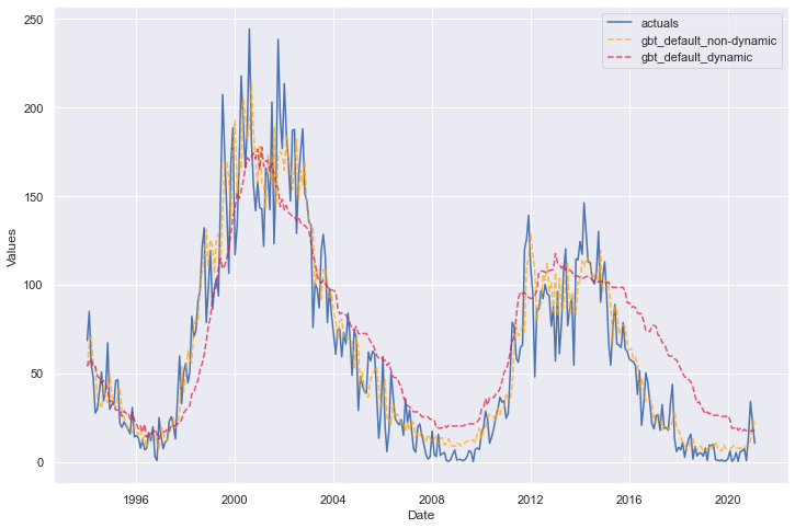
These are the same models trained on the same inputs, but one looks like it performed significantly better than the other. Looks can be deceiving and the model represented by the orange line only did better because it is essentially a string of one-step forecasts whereas the red line is truly out-of-sample for all 326 steps.
So far, we have only seen default parameters for the GBT model. The goal of hyperparameter tuning is to see if a more-optimized model can be found that would produce even better results.
The process of hyperparameter tuning involves training the data on one slice of data and validating it on out-of-sample data (but keeping the test set separate), several times with different hyperparameter combinations each time and selecting the hyperparameters that returned the best performance. There are three ways we can go about this process:
- Train/Validation/Test Split
- Time Series Cross Validation
- Rolling Time Series Cross Validation
Create a Grid
Before employing any of these strategies, we should specify a hyperparameter grid for this model class:
# a simple grid
grid = {
"max_depth": [2, 3, 5, None],
"max_features": ["sqrt", "auto"],
"subsample": [0.8, 0.9, 1],
}
f.ingest_grid(grid)
This grid uses a total of 24 hyperparameter combinations to choose the best model for the task. All three optimization strategies will return a different combination. We then take each of these optimized models to the test set to further evaluate their performance and choose which one we actually believe is best.
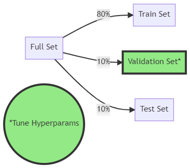
Train/Validation/Test Split
The first optimization strategy is to perform a third split, a validation split, on our data. In this example, we split 10% of our original data and use it as the test set, use 10% in the validation set for hyperparameter optimization, and train the models with the remaining 80%.
This is the simplest and least computationally expensive of the methods we will overview and simply looks like this in code:
f.tune(
dynamic_tuning=True
) # we specified a training/validation/test size earlier
f.auto_forecast(
call_me="gbt_tuned"
) # applies the optimal parameters obtained from tuning
It is important to note, before evaluating on the test set, we retrain the model on the 80% training data combined with the 10% validation data so that the model has seen the most recent observations before it is tested again out of sample. If we don’t retrain the model this way, it will appear to underperform on the test set.
Time Series Cross Validation
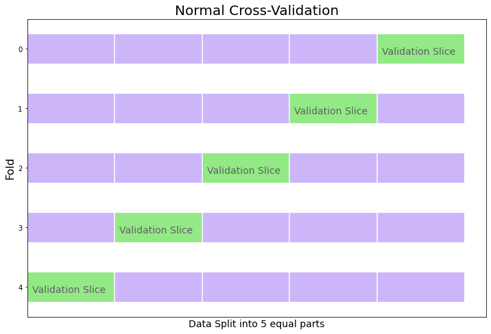
The next strategy is more involved, but could lead to better results, and that is cross validation. On a cross-sectional dataset (not time series), the normal process is to split data into k equally sized subsets (where k can be any integer greater than 1) and train the model k times, each time using the other k-1 subsets of data. We then validate each model from each fold on the remaining validation dataset. The idea is that you can see performance of parameter combinations on several out-of-sample trials to be more certain of a model’s viability. All available data is used to train all models (k-1 times) and all data subsets are also used to test each model (1 time). Errors are then averaged from each out-of-sample trial to come up with a final error metric, which is used to determine the best hyperparameter values.
Cross validation seems complicated the first time you see it, but more complexity can lead to better results, and several libraries make coding this process easy. Below is a diagram where k = 5.
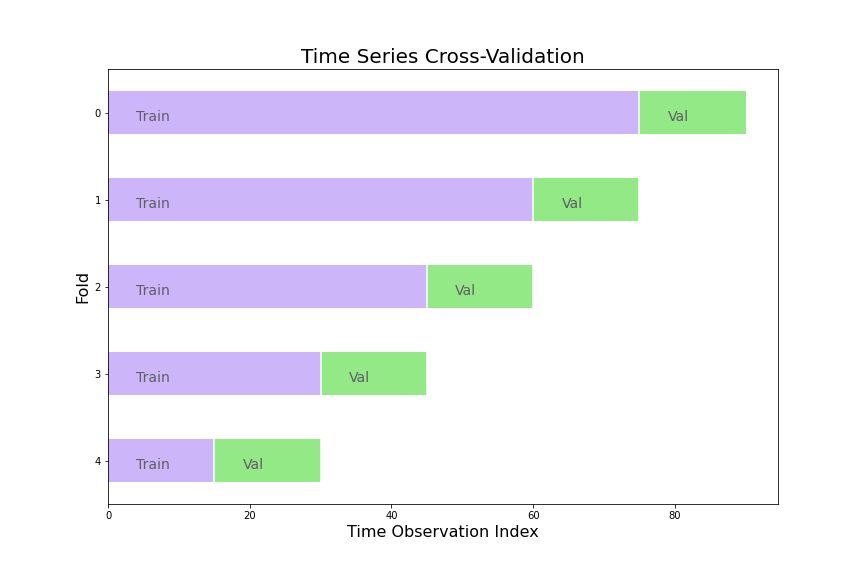
Time series puts a twist on this idea. With any time series model, because the past profoundly impacts the present, the sequence of the data should usually be maintained. We can still use cross validation, but not all data is used to test each model. By the time we get to the last fold, the data used to train the model will never have been tested out-of-sample for the mere reason that there is no data that comes before it sequentially.
Running time series cross validation to tune hyperparameters in code looks like:
f.cross_validate(k=5, dynamic_tuning=True)
f.auto_forecast(call_me="gbt_cv")
Again, after finding the optimal hyperparameters from this process, we retrain the model on the entire training set before dynamically testing it again out-of-sample on the test set, which it has never seen before.
Rolling Time Series Cross Validation
You may realize that a main difference from time series cross validation and regular cross validation is that time series cross validation uses a differently sized training set each time. Therefore, folds with more data may return skewed error metrics compared to folds that have less. To correct for this, we can use a rolling time series cross validation technique:
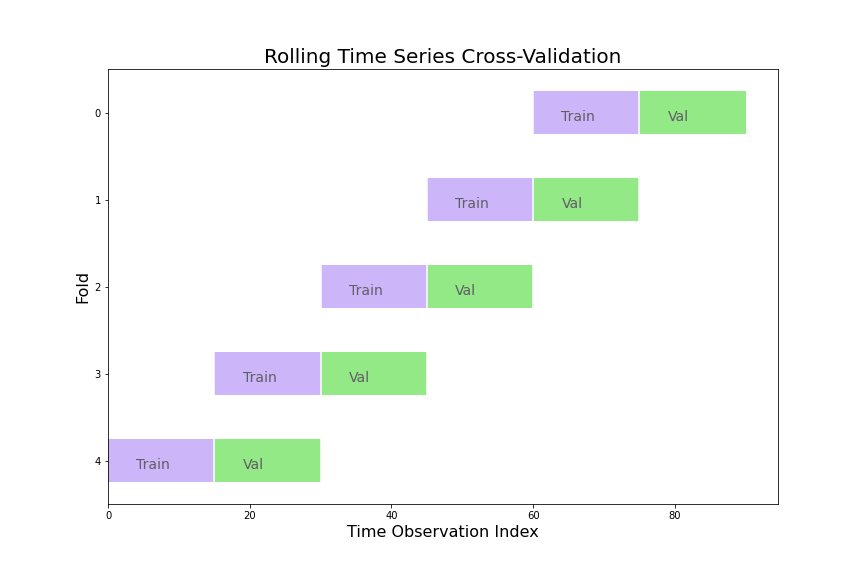
Now every train set and every validation set are the same size, giving more balance to how each fold becomes weighted when averaging the final error. Of course, this comes with a drawback: you have less data to train with in each fold and models and hyperparameters that might benefit from more data will be looked over. All this to say, no one of these strategies is always better than the others and it really comes down to user preference and knowledge of the data being utilized. In code, rolling cross validation looks like this:
f.cross_validate(k=5, rolling=True, dynamic_tuning=True)
f.auto_forecast(call_me="gbt_rolling_cv")
We have now validated our model using three techniques and found three optimal hyperparameter combinations. Each method returned the following optimal hyperparameters:
- Train/validation/test split:
– max_depth: 5
– max_features: ‘sqrt’
– subsample: 1 - Cross validation:
– max_depth: 3
– max_features: ‘sqrt’
– subsample: 1 - Rolling cross validation:
– max_depth: 2
– max_features: ‘auto’
– subsample: 1
We can plot all three of these models together and display the in-sample and out-of-sample error metrics in a table.
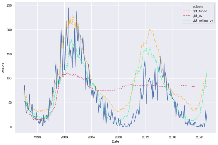
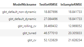
We can ignore the first displayed model, as it was not dynamically tested. The best-performing model, therefore, was the one trained with default hyperparameters. It performs best out-of-sample and shows less evidence of being overfit. However, for the sake of not wanting all of the validation work we did to be in vain and because this is just an example, let’s carry forward the model optimized with rolling cross validation and call that our best model.
best_model = 'gbt_rolling_cv'
One more objective validation we can do on this model is a backtest. Backtesting is for answering the question of how a particular model with a given set of parameters would have performed on the last x-amount of forecast horizons. In our case, let’s say we want to implement this model to predict 10 years (120 periods) into the future. Let’s test it over the last 15 forecast horizons of this size where we know the actual values using only data that came before each of these horizons. Then, let’s look at its average performance across those 15 iterations.
f.backtest(best_model, n_iter=15, fcst_length=120)
f.export_backtest_metrics(best_model)
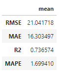
This tells us that on average, we could have seen an RMSE of 21, MAE of 16, and R2 of 74% over a full 120-period forecast window. I would say that is pretty good! You may be wondering why it is so much better than how the test-set metrics suggested it would perform and that is because the test set was almost three-times as large as the 120-period forecast horizon we have now evaluated. It would make sense that the model becomes less effective the further out it is expected to forecast. For this reason, in many applications, it could be a good idea to set the test data size to be the same as the forecast horizon.
The last, and arguably most important, validation step we will employ on this model is the “eye test.” Does the forecast look reasonable into the future horizon? Is it about what we would expect? We can plot the future results and decide:
f.plot(models=best_model,ci=True)
plt.show()
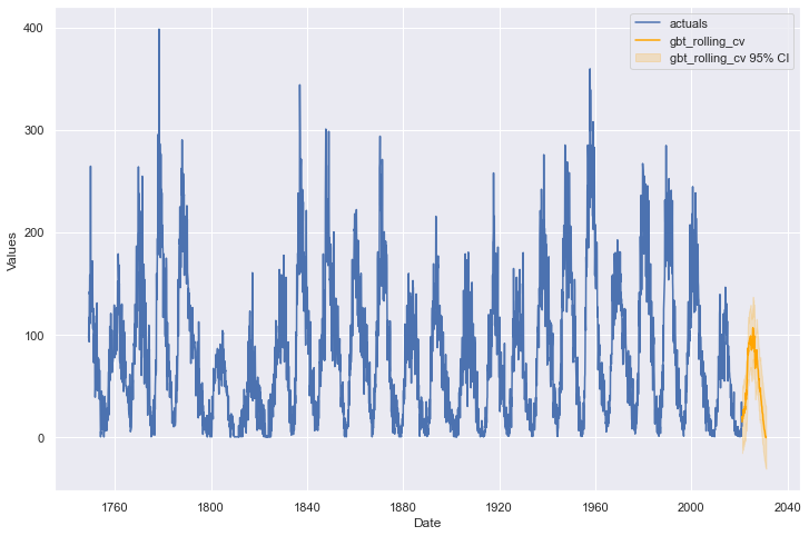
If we think this model looks believable, with all the validation and optimization previously performed, we can feel comfortable about implementing and knowing what to expect from it. I would say we have successfully found and validated an effective time series model!
We now know not only how not to validate a time series model, but what techniques can be employed to successfully optimize a model that can really work. We overviewed dynamic testing, tuning on a validation slice of data, cross validation, rolling cross validation, backtesting, and the eye test. Those are a lot of techniques!
If you found the discussion across the two blog posts interesting, consider checking out scalecast and giving it a star on GitHub. You can also follow me on Medium and sign up for email notifications. Until next time!
Data splitting, cross validation, model optimization, and dynamic predictions to validate forecasting models
How do you know if your time series model is any good? How can you be sure whether changes to your model will make it better or worse? In part 1, we looked at how not validating a model correctly could mislead an audience about its accuracy. In that post, I was seemingly able to predict, among a few other incredible phenomena, COVID-19’s impact on the airline industry only training on data from before 2016, which, if this is not already clear, should not be possible. That post showed what not to do. This post will show what practices should be followed to soundly validate and optimize time-series models.
We first need to do some preparation. We will work with the sunspots dataset, available on Kaggle with a Public Domain license. We employ the following libraries:
If you have an older version of scalecast, cross validation will not be available. It is a good idea to upgrade the package:
pip install scalecast --upgrade
We will be using a 10% test split, leaving 2,939 observations to train and optimize models and 326 observations to test each model we apply. For inputs, we will use the series’ first 120 lags (constituting 10 years of data), a few seasonal lags, several irregular Fourier cycles, and a yearly trend. I talked about feature selection for this same dataset in a previous post. Also in that post, I found that the gradient boosted tree regressor from scikit-learn is a solid estimator of this data, so for brevity’s sake, we will limit the analysis to just that model class.
Find the full notebook here.
To reiterate the lesson learned in Part 1, if you don’t use some kind of dynamic multi-step forecasting procedure to test your model, you can seriously mislead people about the effectiveness of it. If you don’t use a dynamic evaluation technique, you are left with the following options.
Either:
- No lags can be used in the model as inputs unless they are all further in the past from the last known value than the forecast horizon length you are trying to evaluate. In simpler terms, if you are forecasting 10 periods, you can only use the series’ 11th and greater lags as model inputs. You can use other inputs without any problems (such as is the case with the Facebook Prophet model).
Or:
- Model performance must be reported as an average of errors on a string of one-step forecasts and nothing can be claimed to be known about its performance more than one period out.
To drive home this point (and beat a dead horse), let’s call the same model twice using scalecast, once with a dynamic test-set evaluation procedure and once where we reveal the actual values of all autoregressive terms to the model over the entire test set:
f.set_estimator("gbt")
f.manual_forecast(
call_me="gbt_default_non-dynamic",
dynamic_testing=False,
)
f.manual_forecast(
call_me="gbt_default_dynamic"
)  # default is dynamic testing
f.plot_test_set(
models=["gbt_default_non-dynamic", "gbt_default_dynamic"],
include_train=False,
)
plt.show()
These are the same models trained on the same inputs, but one looks like it performed significantly better than the other. Looks can be deceiving and the model represented by the orange line only did better because it is essentially a string of one-step forecasts whereas the red line is truly out-of-sample for all 326 steps.
So far, we have only seen default parameters for the GBT model. The goal of hyperparameter tuning is to see if a more-optimized model can be found that would produce even better results.
The process of hyperparameter tuning involves training the data on one slice of data and validating it on out-of-sample data (but keeping the test set separate), several times with different hyperparameter combinations each time and selecting the hyperparameters that returned the best performance. There are three ways we can go about this process:
- Train/Validation/Test Split
- Time Series Cross Validation
- Rolling Time Series Cross Validation
Create a Grid
Before employing any of these strategies, we should specify a hyperparameter grid for this model class:
# a simple grid
grid = {
"max_depth": [2, 3, 5, None],
"max_features": ["sqrt", "auto"],
"subsample": [0.8, 0.9, 1],
}
f.ingest_grid(grid)
This grid uses a total of 24 hyperparameter combinations to choose the best model for the task. All three optimization strategies will return a different combination. We then take each of these optimized models to the test set to further evaluate their performance and choose which one we actually believe is best.
Train/Validation/Test Split
The first optimization strategy is to perform a third split, a validation split, on our data. In this example, we split 10% of our original data and use it as the test set, use 10% in the validation set for hyperparameter optimization, and train the models with the remaining 80%.
This is the simplest and least computationally expensive of the methods we will overview and simply looks like this in code:
f.tune(
dynamic_tuning=True
) # we specified a training/validation/test size earlier
f.auto_forecast(
call_me="gbt_tuned"
) # applies the optimal parameters obtained from tuning
It is important to note, before evaluating on the test set, we retrain the model on the 80% training data combined with the 10% validation data so that the model has seen the most recent observations before it is tested again out of sample. If we don’t retrain the model this way, it will appear to underperform on the test set.
Time Series Cross Validation
The next strategy is more involved, but could lead to better results, and that is cross validation. On a cross-sectional dataset (not time series), the normal process is to split data into k equally sized subsets (where k can be any integer greater than 1) and train the model k times, each time using the other k-1 subsets of data. We then validate each model from each fold on the remaining validation dataset. The idea is that you can see performance of parameter combinations on several out-of-sample trials to be more certain of a model’s viability. All available data is used to train all models (k-1 times) and all data subsets are also used to test each model (1 time). Errors are then averaged from each out-of-sample trial to come up with a final error metric, which is used to determine the best hyperparameter values.
Cross validation seems complicated the first time you see it, but more complexity can lead to better results, and several libraries make coding this process easy. Below is a diagram where k = 5.
Time series puts a twist on this idea. With any time series model, because the past profoundly impacts the present, the sequence of the data should usually be maintained. We can still use cross validation, but not all data is used to test each model. By the time we get to the last fold, the data used to train the model will never have been tested out-of-sample for the mere reason that there is no data that comes before it sequentially.
Running time series cross validation to tune hyperparameters in code looks like:
f.cross_validate(k=5, dynamic_tuning=True)
f.auto_forecast(call_me="gbt_cv")
Again, after finding the optimal hyperparameters from this process, we retrain the model on the entire training set before dynamically testing it again out-of-sample on the test set, which it has never seen before.
Rolling Time Series Cross Validation
You may realize that a main difference from time series cross validation and regular cross validation is that time series cross validation uses a differently sized training set each time. Therefore, folds with more data may return skewed error metrics compared to folds that have less. To correct for this, we can use a rolling time series cross validation technique:
Now every train set and every validation set are the same size, giving more balance to how each fold becomes weighted when averaging the final error. Of course, this comes with a drawback: you have less data to train with in each fold and models and hyperparameters that might benefit from more data will be looked over. All this to say, no one of these strategies is always better than the others and it really comes down to user preference and knowledge of the data being utilized. In code, rolling cross validation looks like this:
f.cross_validate(k=5, rolling=True, dynamic_tuning=True)
f.auto_forecast(call_me="gbt_rolling_cv")
We have now validated our model using three techniques and found three optimal hyperparameter combinations. Each method returned the following optimal hyperparameters:
- Train/validation/test split:
– max_depth: 5
– max_features: ‘sqrt’
– subsample: 1 - Cross validation:
– max_depth: 3
– max_features: ‘sqrt’
– subsample: 1 - Rolling cross validation:
– max_depth: 2
– max_features: ‘auto’
– subsample: 1
We can plot all three of these models together and display the in-sample and out-of-sample error metrics in a table.
We can ignore the first displayed model, as it was not dynamically tested. The best-performing model, therefore, was the one trained with default hyperparameters. It performs best out-of-sample and shows less evidence of being overfit. However, for the sake of not wanting all of the validation work we did to be in vain and because this is just an example, let’s carry forward the model optimized with rolling cross validation and call that our best model.
best_model = 'gbt_rolling_cv'
One more objective validation we can do on this model is a backtest. Backtesting is for answering the question of how a particular model with a given set of parameters would have performed on the last x-amount of forecast horizons. In our case, let’s say we want to implement this model to predict 10 years (120 periods) into the future. Let’s test it over the last 15 forecast horizons of this size where we know the actual values using only data that came before each of these horizons. Then, let’s look at its average performance across those 15 iterations.
f.backtest(best_model, n_iter=15, fcst_length=120)
f.export_backtest_metrics(best_model)
This tells us that on average, we could have seen an RMSE of 21, MAE of 16, and R2 of 74% over a full 120-period forecast window. I would say that is pretty good! You may be wondering why it is so much better than how the test-set metrics suggested it would perform and that is because the test set was almost three-times as large as the 120-period forecast horizon we have now evaluated. It would make sense that the model becomes less effective the further out it is expected to forecast. For this reason, in many applications, it could be a good idea to set the test data size to be the same as the forecast horizon.
The last, and arguably most important, validation step we will employ on this model is the “eye test.” Does the forecast look reasonable into the future horizon? Is it about what we would expect? We can plot the future results and decide:
f.plot(models=best_model,ci=True)
plt.show()
If we think this model looks believable, with all the validation and optimization previously performed, we can feel comfortable about implementing and knowing what to expect from it. I would say we have successfully found and validated an effective time series model!
We now know not only how not to validate a time series model, but what techniques can be employed to successfully optimize a model that can really work. We overviewed dynamic testing, tuning on a validation slice of data, cross validation, rolling cross validation, backtesting, and the eye test. Those are a lot of techniques!
If you found the discussion across the two blog posts interesting, consider checking out scalecast and giving it a star on GitHub. You can also follow me on Medium and sign up for email notifications. Until next time!
Denial of responsibility! Techno Blender is an automatic aggregator of the all world’s media. In each content, the hyperlink to the primary source is specified. All trademarks belong to their rightful owners, all materials to their authors. If you are the owner of the content and do not want us to publish your materials, please contact us by email – [email protected]. The content will be deleted within 24 hours.