Three Critical Elements of Data Preprocessing — Part 2 | by Abiodun Olaoye | Oct, 2022

The backbone of modeling in data science

Data preprocessing is one of the main steps in the data science project life cycle which involves converting raw data into a refined form amenable to data analysis.

In the first article of this series, I covered the data integration component of data preprocessing which involves combining data from disparate sources to obtain a dataset consisting of all available relevant features and examples. The link to the article can be found here:

In this article, I will discuss the next component of data preprocessing and perhaps the most critical for modeling purposes known as data cleaning. In addition, I will share resources for tackling different sections of the data-cleaning process.

This is the process of identifying and removing or correcting duplicated, corrupted, and missing data from a collected dataset.

Data cleaning improves the quality of data fed to machine learning algorithms and can make or break a data science project. Although typically a time-consuming process, data cleaning yields great benefits especially in improving model performance since a model is only as good as the data it receives.

Hence, generating cleaner data is better than spending more computing power and time tuning sophisticated algorithms.

The data-cleaning process consists of the following tasks:

Correcting structural errors

This involves identifying and fixing inconsistencies in the data. For example, categorical features may be labeled with different capitalization (Male vs male) or target variables may be assigned to the wrong class. The latter is hard to detect and may require domain expert knowledge to uncover.

The value_counts method in Pandas DataFrame can be used to investigate the unique labels in each column of the dataset. Also, a bar chart of unique label counts can be used for visual inspection of inconsistencies in the data.

Resources:

Data cleaning — https://www.tableau.com/learn/articles/what-is-data-cleaning#:~:text=Data%20cleaning%20is%20the%20process,to%20be%20duplicated%20or%20mislabeled.

Pandas value counts — https://pandas.pydata.org/pandas-docs/stable/reference/api/pandas.DataFrame.value_counts.html

Handling missing values

Depending on the prevalence and type of missing values being dealt with, missing values may be estimated or affected observations (examples) may be removed.

Based on experience, I will suggest dropping observations when the percentage of missing values is “very small” (say < 5%) compared with overall available data. Similarly, features with more than 95% of the data missing may be dropped although these are hard not thresholds and can be changed based on domain knowledge.

Missing values occur in several forms including:

(1) Missing completely at random (MCAR): In this case, the missing data is independent of the observed or unobserved samples and does not introduce bias. Hence, they can be removed. However, the proportion of the total population that can be analyzed is reduced.

(2) Missing at random (MAR): Here, the missing data is dependent on the observed data. For example, missing values that are affected by attributes of the observed data such as age or gender may occur randomly but may or may not introduce bias in the dataset. These values can be imputed using interpolation or other statistical estimates based on observed data.

(3) Missing not at random (MNAR): In this case, the missing data is dependent on the unobserved data, and insights from such datasets are more likely to be biased. These missing values are typically non-ignorable and cannot be imputed by standard methods hence, they are highly problematic to analyze. On the other hand, there is a class of MNAR known as structurally missing data which are analyzable.

Resources:

Tackling outliers

Outliers are data points that exist outside the expected range of values for a given variable. As defined, the expected range is subjective and depends on the field of investigation.

However, there are ways of handling outliers including outright elimination of affected data points, clipping the values to a certain threshold based on data distribution, and estimating the actual value of the data point (treating the point as a missing value).

All outliers are not created equal. Some are simply noise that distracts your machine-learning models, while others are a representation of your data’s real-world attributes.

Eliminating a “good” outlier may jeopardize the data cleaning process and result in unrepresentative data models.

Domain knowledge and expert consultation are good ways to spot the difference.

How do you detect outliers? Here is a list of methods for detecting outliers:

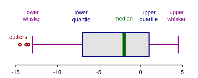
(1) Data visualizations: Boxplots and histograms are useful for quickly identifying outliers in the data. Many plotting tools such as Seaborn, Tableau, and Power BI have the functionality to create these graphs.

(2) Standard deviation thresholds: For approximately normally distributed data, outliers can be defined as data points that are +/ — x standard deviations from the mean. Where the value of x typically ranges from 1 to 3 depending on the field of application.

(3) Interquartile range thresholds: An outlier may be defined as data points existing outside 1.5 times the interquartile range (1.5*IQR) in both positive and negative directions. Where the interquartile range is the distance between the third (upper) quartile and the first (lower) quartile. The threshold may be increased to 3*IQR to detect extreme outliers.

(4) Hypothesis testing: Statistical tests may be used to detect the presence of outliers in a dataset depending on the data distribution. Some examples include Grubb’s test, Dixon’s Q test, and the Chi-square test. In this approach, the null hypothesis states that there are no outliers in the data while the alternative hypothesis states that there is at least one outlier. With a significance level, α (say 0.05), the null hypothesis is rejected if the P-value of the test is less than α and it is inferred that an outlier exists.

(5) Anomaly detection models: Both supervised and unsupervised machine learning models may be built to learn the typical values of a variable based on other predictive features in the datasets. However, this approach can be computationally expensive and even excessive.

Resources:

Methods for identifying outliers — https://statisticsbyjim.com/basics/outliers/

Hypothesis testing for outlier detection — https://www.dummies.com/article/technology/information-technology/data-science/big-data/hypothesis-tests-for-data-outliers-141226/

Removal of wrong observations

During data integration, some observations may be duplicated or corrupted. Eliminating affected data points helps to avoid misrepresentation of the data patterns or issues such as overfitting during modeling. Hence, cleaning up wrong data points can significantly improve model performance.

In this article, I covered data cleaning, a critical element of data preprocessing. As we have seen, this process is quite involved but it pays a significant dividend in model performance improvement.

In the next and final article of this series, I will discuss data transformation which also includes data reduction strategies.

I hope you have enjoyed this series so far, until next time. Cheers!

The backbone of modeling in data science

Data preprocessing is one of the main steps in the data science project life cycle which involves converting raw data into a refined form amenable to data analysis.

In the first article of this series, I covered the data integration component of data preprocessing which involves combining data from disparate sources to obtain a dataset consisting of all available relevant features and examples. The link to the article can be found here:

In this article, I will discuss the next component of data preprocessing and perhaps the most critical for modeling purposes known as data cleaning. In addition, I will share resources for tackling different sections of the data-cleaning process.

This is the process of identifying and removing or correcting duplicated, corrupted, and missing data from a collected dataset.

Data cleaning improves the quality of data fed to machine learning algorithms and can make or break a data science project. Although typically a time-consuming process, data cleaning yields great benefits especially in improving model performance since a model is only as good as the data it receives.

Hence, generating cleaner data is better than spending more computing power and time tuning sophisticated algorithms.

The data-cleaning process consists of the following tasks:

Correcting structural errors

This involves identifying and fixing inconsistencies in the data. For example, categorical features may be labeled with different capitalization (Male vs male) or target variables may be assigned to the wrong class. The latter is hard to detect and may require domain expert knowledge to uncover.

The value_counts method in Pandas DataFrame can be used to investigate the unique labels in each column of the dataset. Also, a bar chart of unique label counts can be used for visual inspection of inconsistencies in the data.

Resources:

Data cleaning — https://www.tableau.com/learn/articles/what-is-data-cleaning#:~:text=Data%20cleaning%20is%20the%20process,to%20be%20duplicated%20or%20mislabeled.

Pandas value counts — https://pandas.pydata.org/pandas-docs/stable/reference/api/pandas.DataFrame.value_counts.html

Handling missing values

Depending on the prevalence and type of missing values being dealt with, missing values may be estimated or affected observations (examples) may be removed.

Based on experience, I will suggest dropping observations when the percentage of missing values is “very small” (say < 5%) compared with overall available data. Similarly, features with more than 95% of the data missing may be dropped although these are hard not thresholds and can be changed based on domain knowledge.

Missing values occur in several forms including:

(1) Missing completely at random (MCAR): In this case, the missing data is independent of the observed or unobserved samples and does not introduce bias. Hence, they can be removed. However, the proportion of the total population that can be analyzed is reduced.

(2) Missing at random (MAR): Here, the missing data is dependent on the observed data. For example, missing values that are affected by attributes of the observed data such as age or gender may occur randomly but may or may not introduce bias in the dataset. These values can be imputed using interpolation or other statistical estimates based on observed data.

(3) Missing not at random (MNAR): In this case, the missing data is dependent on the unobserved data, and insights from such datasets are more likely to be biased. These missing values are typically non-ignorable and cannot be imputed by standard methods hence, they are highly problematic to analyze. On the other hand, there is a class of MNAR known as structurally missing data which are analyzable.

Resources:

Tackling outliers

Outliers are data points that exist outside the expected range of values for a given variable. As defined, the expected range is subjective and depends on the field of investigation.

However, there are ways of handling outliers including outright elimination of affected data points, clipping the values to a certain threshold based on data distribution, and estimating the actual value of the data point (treating the point as a missing value).

All outliers are not created equal. Some are simply noise that distracts your machine-learning models, while others are a representation of your data’s real-world attributes.

Eliminating a “good” outlier may jeopardize the data cleaning process and result in unrepresentative data models.

Domain knowledge and expert consultation are good ways to spot the difference.

How do you detect outliers? Here is a list of methods for detecting outliers:

(1) Data visualizations: Boxplots and histograms are useful for quickly identifying outliers in the data. Many plotting tools such as Seaborn, Tableau, and Power BI have the functionality to create these graphs.

(2) Standard deviation thresholds: For approximately normally distributed data, outliers can be defined as data points that are +/ — x standard deviations from the mean. Where the value of x typically ranges from 1 to 3 depending on the field of application.

(3) Interquartile range thresholds: An outlier may be defined as data points existing outside 1.5 times the interquartile range (1.5*IQR) in both positive and negative directions. Where the interquartile range is the distance between the third (upper) quartile and the first (lower) quartile. The threshold may be increased to 3*IQR to detect extreme outliers.

(4) Hypothesis testing: Statistical tests may be used to detect the presence of outliers in a dataset depending on the data distribution. Some examples include Grubb’s test, Dixon’s Q test, and the Chi-square test. In this approach, the null hypothesis states that there are no outliers in the data while the alternative hypothesis states that there is at least one outlier. With a significance level, α (say 0.05), the null hypothesis is rejected if the P-value of the test is less than α and it is inferred that an outlier exists.

(5) Anomaly detection models: Both supervised and unsupervised machine learning models may be built to learn the typical values of a variable based on other predictive features in the datasets. However, this approach can be computationally expensive and even excessive.

Resources:

Methods for identifying outliers — https://statisticsbyjim.com/basics/outliers/

Hypothesis testing for outlier detection — https://www.dummies.com/article/technology/information-technology/data-science/big-data/hypothesis-tests-for-data-outliers-141226/

Removal of wrong observations

During data integration, some observations may be duplicated or corrupted. Eliminating affected data points helps to avoid misrepresentation of the data patterns or issues such as overfitting during modeling. Hence, cleaning up wrong data points can significantly improve model performance.

In this article, I covered data cleaning, a critical element of data preprocessing. As we have seen, this process is quite involved but it pays a significant dividend in model performance improvement.

In the next and final article of this series, I will discuss data transformation which also includes data reduction strategies.

I hope you have enjoyed this series so far, until next time. Cheers!