
Time Series Classification with LightGBM | by Tyler Blume | Jul, 2022
An example using LazyProphet
Classification is a common task when dealing with time series data. This task is made difficult by the presence of trends and seasonality, similar to time series regression. Luckily, the same features derived for regression with LightGBM can be useful for classification as well. This task is then made easy by using LazyProphet.
This article is a follow-up to my previous review of LazyProphet:
In that article, we tackled the standard time series regression problem and achieved state-of-the-art (I think) results for univariate time series trees on the M4 dataset. The key lies in utilizing linear-piecewise basis functions. While not all that unique, we add a twist — the functions are weighted to fit the data better. This enables the trees to achieve significantly better performance. If you are confused as to what those are, definitely check out the previous article!
Additionally, LazyProphet provides functionality to forecast ‘recursively’, that is, forecasting using previous target values. This requires that we use future predictions at some point in the process, which is a tad annoying to code and handle from scratch.
Finally, there are also some unique ways we think about trends in the case of trees that aid in the improvements as well, you can check out an article about that here:
Luckily for us, these same techniques can be applied to solve classification problems as well. In this article, we will take a quick look at solving one such problem with LazyProphet.
But first, if you haven’t installed the package yet, it is only a pip away:
pip install LazyProphet
Now, let’s get to the data.
For this example we will use an example from Scikit-Learn’s open datasets: The Bike Sharing Demand dataset.
from sklearn.datasets import fetch_openml
import matplotlib.pyplot as plt
import seaborn as sns
sns.set_style('darkgrid')bike_sharing = fetch_openml("Bike_Sharing_Demand", version=2, as_frame=True)
y = bike_sharing.frame['count']
y = y[-800:].values
plt.plot(y)
plt.show()

Obviously, this data isn’t made for a binary classification so let’s fix that.
y_class = y > 70
y_class = y_class * 1
plt.plot(y_class)
plt.show()
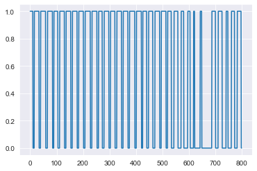
Here we are simply labelling any value over 70 as 1’s and all values below as 0’s. There is clearly some seasonality, as well as some ‘shocks’ between 600 and 700 hours.
Next, we simply build the model:
from LazyProphet import LazyProphet as lplp_model = lp.LazyProphet(seasonal_period=[24],
n_basis=10,
objective='classification',
fourier_order=5,
decay=.99,
ar=3,
return_proba=True)
seasonal_period— The seasonality of the data. We can pass an int or float as well as a list. If we pass a list, we can pass multiple values for complex seasonality such as[7, 365.25].n_basis— The number of piecewise basis functions to use. This is used to measure ‘trends’ as well as allow the seasonality to change over time.objective— Either'classification'or'regression'. If we passclassificationthen LazyProphet uses a binary cross entropy objective function. If we passregressionthen LazyProphet uses the RMSE.fourier_order— The number of sine and cosine components used to approximate the seasonal pulse. The higher the number the more wiggly the fit it!decay— The ‘decay’ or penalty weight on our trend basis functions. If you don’t know what this is then check out the aforementioned article.ar— The number of past values used to predict with. If we pass an int here then LazyProphet automatically does one-step predictions and uses that prediction for the next step for the entire forecast horizon.return_proba— Boolean flag, if set toTruethen LazyProphet returns the probabilities and, ifFalse, just the [1, 0] classifications.
Now we just need to fit the model to our data and predict 100 steps:
fitted = lp_model.fit(y_class)
predicted_class = lp_model.predict(100)
plt.plot(y_class)
plt.plot(np.append(fitted, predicted_class), alpha=.5)
plt.axvline(800)
plt.show()

Voilà!
We have a reasonable forecast of the probabilities. Of course, tree models fit the training data unreasonably well, so we should be careful about evaluating our fit. Further iterations can be done with different hyperparameters.
Sometimes (such as in this example) our labels are derived or are heavily correlated to a time series with real numbers, not binary ones. If this is the case, we simply need to pass that series when building the model object. That will look like this:
lp_model = lp.LazyProphet(seasonal_period=[24],
n_basis=3,
objective='classification',
fourier_order=5,
decay=.99,
#ar=3, ar should be turned off here
return_proba=True,
series_features=y,
)
Where ‘y’ is our original series we manipulated into the binary classification labels. Note that ar needs to be disabled. From here, the rest of the procedure is the same!
In this article we took a stab at time series classification with LazyProphet. Since the core is built with LightGBM, switching from a regression problem to a classification one is quite easy. But, the real performance gains we see come from the weighted basis functions.
Make sure to check out the github and open any issues you come across!
If you enjoyed this article you may enjoy a few others I have written:
And you can buy me a coffee by joining Medium through my referral link:
An example using LazyProphet

Classification is a common task when dealing with time series data. This task is made difficult by the presence of trends and seasonality, similar to time series regression. Luckily, the same features derived for regression with LightGBM can be useful for classification as well. This task is then made easy by using LazyProphet.
This article is a follow-up to my previous review of LazyProphet:
In that article, we tackled the standard time series regression problem and achieved state-of-the-art (I think) results for univariate time series trees on the M4 dataset. The key lies in utilizing linear-piecewise basis functions. While not all that unique, we add a twist — the functions are weighted to fit the data better. This enables the trees to achieve significantly better performance. If you are confused as to what those are, definitely check out the previous article!
Additionally, LazyProphet provides functionality to forecast ‘recursively’, that is, forecasting using previous target values. This requires that we use future predictions at some point in the process, which is a tad annoying to code and handle from scratch.
Finally, there are also some unique ways we think about trends in the case of trees that aid in the improvements as well, you can check out an article about that here:
Luckily for us, these same techniques can be applied to solve classification problems as well. In this article, we will take a quick look at solving one such problem with LazyProphet.
But first, if you haven’t installed the package yet, it is only a pip away:
pip install LazyProphet
Now, let’s get to the data.
For this example we will use an example from Scikit-Learn’s open datasets: The Bike Sharing Demand dataset.
from sklearn.datasets import fetch_openml
import matplotlib.pyplot as plt
import seaborn as sns
sns.set_style('darkgrid')bike_sharing = fetch_openml("Bike_Sharing_Demand", version=2, as_frame=True)
y = bike_sharing.frame['count']
y = y[-800:].values
plt.plot(y)
plt.show()
Obviously, this data isn’t made for a binary classification so let’s fix that.
y_class = y > 70
y_class = y_class * 1
plt.plot(y_class)
plt.show()
Here we are simply labelling any value over 70 as 1’s and all values below as 0’s. There is clearly some seasonality, as well as some ‘shocks’ between 600 and 700 hours.
Next, we simply build the model:
from LazyProphet import LazyProphet as lplp_model = lp.LazyProphet(seasonal_period=[24],
n_basis=10,
objective='classification',
fourier_order=5,
decay=.99,
ar=3,
return_proba=True)
seasonal_period— The seasonality of the data. We can pass an int or float as well as a list. If we pass a list, we can pass multiple values for complex seasonality such as[7, 365.25].n_basis— The number of piecewise basis functions to use. This is used to measure ‘trends’ as well as allow the seasonality to change over time.objective— Either'classification'or'regression'. If we passclassificationthen LazyProphet uses a binary cross entropy objective function. If we passregressionthen LazyProphet uses the RMSE.fourier_order— The number of sine and cosine components used to approximate the seasonal pulse. The higher the number the more wiggly the fit it!decay— The ‘decay’ or penalty weight on our trend basis functions. If you don’t know what this is then check out the aforementioned article.ar— The number of past values used to predict with. If we pass an int here then LazyProphet automatically does one-step predictions and uses that prediction for the next step for the entire forecast horizon.return_proba— Boolean flag, if set toTruethen LazyProphet returns the probabilities and, ifFalse, just the [1, 0] classifications.
Now we just need to fit the model to our data and predict 100 steps:
fitted = lp_model.fit(y_class)
predicted_class = lp_model.predict(100)
plt.plot(y_class)
plt.plot(np.append(fitted, predicted_class), alpha=.5)
plt.axvline(800)
plt.show()
Voilà!
We have a reasonable forecast of the probabilities. Of course, tree models fit the training data unreasonably well, so we should be careful about evaluating our fit. Further iterations can be done with different hyperparameters.
Sometimes (such as in this example) our labels are derived or are heavily correlated to a time series with real numbers, not binary ones. If this is the case, we simply need to pass that series when building the model object. That will look like this:
lp_model = lp.LazyProphet(seasonal_period=[24],
n_basis=3,
objective='classification',
fourier_order=5,
decay=.99,
#ar=3, ar should be turned off here
return_proba=True,
series_features=y,
)
Where ‘y’ is our original series we manipulated into the binary classification labels. Note that ar needs to be disabled. From here, the rest of the procedure is the same!
In this article we took a stab at time series classification with LazyProphet. Since the core is built with LightGBM, switching from a regression problem to a classification one is quite easy. But, the real performance gains we see come from the weighted basis functions.
Make sure to check out the github and open any issues you come across!
If you enjoyed this article you may enjoy a few others I have written:
And you can buy me a coffee by joining Medium through my referral link:
Denial of responsibility! Techno Blender is an automatic aggregator of the all world’s media. In each content, the hyperlink to the primary source is specified. All trademarks belong to their rightful owners, all materials to their authors. If you are the owner of the content and do not want us to publish your materials, please contact us by email – [email protected]. The content will be deleted within 24 hours.