
3-Step Feature Selection Guide in Sklearn to Superchage Your Models | by Bex T. | Oct, 2022
Develop a robust Feature Selection workflow for any supervised problem
Learn how to face one of the biggest challenges of machine learning with the best of Sklearn feature selectors.
Introduction
Today, it is common for datasets to have hundreds if not thousands of features. On the surface, this might seem like a good thing — more features give more information about each sample. But more often than not, these additional features don’t provide much value and introduce complexity.
The biggest challenge of Machine Learning is to create models that have robust predictive power by using as few features as possible. But given the massive sizes of today’s datasets, it is easy to lose the oversight of which features are important and which ones aren’t.
That’s why there is an entire skill to be learned in the ML field — feature selection. Feature selection is the process of choosing a subset of the most important features while trying to retain as much information as possible (An excerpt from the first article in this series).
As feature selection is such a pressing issue, there is a myriad of solutions you can select from🤦♂️🤦♂️. To spare you some pain, I will teach you 3feature selection techniques that, when used together, can supercharge any model’s performance.
This article will give you an overview of these techniques and how to use them without wondering too much about the internals. For a deeper understanding, I have written separate posts for each with the nitty-gritty explained. Let’s get started!
Intro to the dataset and the problem statement
We will be working with the Ansur Male dataset, which contains more than 100 different US Army personnel body measurements. I have been using this dataset excessively throughout this feature selection series because it contains 98 numeric features — a perfect dataset to teach feature selection.

We will be trying to predict the weight in pounds, so it is a regression problem. Let’s establish a base performance with simple Linear Regression. LR is a good candidate for this problem because we can expect body measurements to be linearly correlated:
For the base performance, we got an impressive R-squared of 0.956. However, this might be because there is also weight in kilograms column among features, giving the algorithm all it needs (we are trying to predict weight in pounds). So, let’s try without it:
Now, we have 0.945, but we managed to reduce model complexity.
Step I: Variance Thresholding
The first technique will be targeted at the individual properties of each feature. The idea behind Variance Thresholding is that features with low variance do not contribute much to overall predictions. These types of features have distributions with too few unique values or low-enough variances to make no matter. VT helps us to remove them using Sklearn.
One concern before applying VT is the scale of features. As the values in a feature get bigger, the variance grows exponentially. This means that features with different distributions have different scales, so we cannot safely compare their variances. So, we must apply some form of normalization to bring all features to the same scale and then apply VT. Here is the code:
After normalization (here, we are dividing each sample by the feature’s mean), you should choose a threshold between 0 and 1. Instead of using the .transform() method of the VT estimator, we are using get_support() which gives a boolean mask (True values for features that should be kept). Then, it can be used to subset the data while preserving the column names.
This may be a simple technique, but it can go a long in eliminating useless features. For deeper insight and more explanation of the code, you can head over to this article:
Step II: Pairwise Correlation
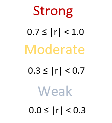
We will further trim our dataset by focusing on the relationships between features. One of the best metrics that show a linear connection is Pearson’s correlation coefficient (denoted r). The logic behind using r for feature selection is simple. If the correlation between features A and B is 0.9, it means you can predict the values of B using the values of A 90% of the time. In other words, in a dataset where A is present, you can discard B or vice versa.
There isn’t a Sklearn estimator that implements feature selection based on correlation. So, we will do it on our own:
This function is a shorthand that returns the names of columns that should be dropped based on a custom correlation threshold. Usually, the threshold will be over 0.8 to be safe.
In the function, we first create a correlation matrix using .corr(). Next, we create a boolean mask to only include correlations below the correlation matrix’s diagonal. We use this mask to subset the matrix. Finally, in a list comprehension, we find the names of features that should be dropped and return them.
There is a lot I didn’t explain about the code. Even though this function works well, I suggest reading my separate article on feature selection based on the correlation coefficient. I fully explained the concept of correlation and how it is different from causation. There is also a separate section on plotting the perfect correlation matrix as a heatmap and, of course, the explanation of the above function.
For our dataset, we will choose a threshold of 0.9:
The function tells us to drop 13 features:
Now, only 35 features are remaining.
Step III: Recursive Feature Elimination with Cross-Validation (RFECV)
Finally, we will choose the final set of features based on how they affect model performance. Most of the Sklearn models have either .coef_ (linear models) or .feature_importances_ (tree-based and ensemble models) attributes that show the importance of each feature. For example, let’s fit the Linear Regression model to the current set of features and see the computed coefficients:

The above DataFrame shows the features with the smallest coefficients. The smaller the weight or the coefficient of a feature is, the less it contributes to the model’s predictive power. With this idea in mind, Recursive Feature Elimination removes features one-by-one using cross-validation until the best smallest set of features is remaining.
Sklearn implements this technique under the RFECV class which takes an arbitrary estimator and several other arguments:
After fitting the estimator to the data, we can get a boolean mask with True values encoding the features that should be kept. We can finally use it to subset the original data one last time:
After applying RFECV, we managed to discard 5 more features. Let’s evaluate a final GradientBoostingRegressor model on this feature selected dataset and see its performance:
Even though we got a slight drop in performance, we managed to remove almost 70 features reducing model complexity significantly.
In a separate article, I further discussed the .coef_ and .feature_importances_ attributes as well as extra details of what happens in each elimination round of RFE:
Summary
Feature selection should not be taken lightly. While reducing model complexity, some algorithms can even see an increase in the performance due to the lack of distracting features in the dataset. It is also not wise to rely on a single method. Instead, approach the problem from different angles and using various techniques.
Today, we saw how to apply feature selection to a dataset in three stages:
- Based on the properties of each feature using Variance Thresholding.
- Based on the relationships between features using Pairwise Correlation.
- Based on how features affect a model’s performance.
Using these techniques in procession should give you reliable results for any supervised problem you face.
Further Reading on Feature Selection
Develop a robust Feature Selection workflow for any supervised problem
Learn how to face one of the biggest challenges of machine learning with the best of Sklearn feature selectors.

Introduction
Today, it is common for datasets to have hundreds if not thousands of features. On the surface, this might seem like a good thing — more features give more information about each sample. But more often than not, these additional features don’t provide much value and introduce complexity.
The biggest challenge of Machine Learning is to create models that have robust predictive power by using as few features as possible. But given the massive sizes of today’s datasets, it is easy to lose the oversight of which features are important and which ones aren’t.
That’s why there is an entire skill to be learned in the ML field — feature selection. Feature selection is the process of choosing a subset of the most important features while trying to retain as much information as possible (An excerpt from the first article in this series).
As feature selection is such a pressing issue, there is a myriad of solutions you can select from🤦♂️🤦♂️. To spare you some pain, I will teach you 3feature selection techniques that, when used together, can supercharge any model’s performance.
This article will give you an overview of these techniques and how to use them without wondering too much about the internals. For a deeper understanding, I have written separate posts for each with the nitty-gritty explained. Let’s get started!
Intro to the dataset and the problem statement
We will be working with the Ansur Male dataset, which contains more than 100 different US Army personnel body measurements. I have been using this dataset excessively throughout this feature selection series because it contains 98 numeric features — a perfect dataset to teach feature selection.
We will be trying to predict the weight in pounds, so it is a regression problem. Let’s establish a base performance with simple Linear Regression. LR is a good candidate for this problem because we can expect body measurements to be linearly correlated:
For the base performance, we got an impressive R-squared of 0.956. However, this might be because there is also weight in kilograms column among features, giving the algorithm all it needs (we are trying to predict weight in pounds). So, let’s try without it:
Now, we have 0.945, but we managed to reduce model complexity.
Step I: Variance Thresholding
The first technique will be targeted at the individual properties of each feature. The idea behind Variance Thresholding is that features with low variance do not contribute much to overall predictions. These types of features have distributions with too few unique values or low-enough variances to make no matter. VT helps us to remove them using Sklearn.
One concern before applying VT is the scale of features. As the values in a feature get bigger, the variance grows exponentially. This means that features with different distributions have different scales, so we cannot safely compare their variances. So, we must apply some form of normalization to bring all features to the same scale and then apply VT. Here is the code:
After normalization (here, we are dividing each sample by the feature’s mean), you should choose a threshold between 0 and 1. Instead of using the .transform() method of the VT estimator, we are using get_support() which gives a boolean mask (True values for features that should be kept). Then, it can be used to subset the data while preserving the column names.
This may be a simple technique, but it can go a long in eliminating useless features. For deeper insight and more explanation of the code, you can head over to this article:
Step II: Pairwise Correlation
We will further trim our dataset by focusing on the relationships between features. One of the best metrics that show a linear connection is Pearson’s correlation coefficient (denoted r). The logic behind using r for feature selection is simple. If the correlation between features A and B is 0.9, it means you can predict the values of B using the values of A 90% of the time. In other words, in a dataset where A is present, you can discard B or vice versa.
There isn’t a Sklearn estimator that implements feature selection based on correlation. So, we will do it on our own:
This function is a shorthand that returns the names of columns that should be dropped based on a custom correlation threshold. Usually, the threshold will be over 0.8 to be safe.
In the function, we first create a correlation matrix using .corr(). Next, we create a boolean mask to only include correlations below the correlation matrix’s diagonal. We use this mask to subset the matrix. Finally, in a list comprehension, we find the names of features that should be dropped and return them.
There is a lot I didn’t explain about the code. Even though this function works well, I suggest reading my separate article on feature selection based on the correlation coefficient. I fully explained the concept of correlation and how it is different from causation. There is also a separate section on plotting the perfect correlation matrix as a heatmap and, of course, the explanation of the above function.
For our dataset, we will choose a threshold of 0.9:
The function tells us to drop 13 features:
Now, only 35 features are remaining.
Step III: Recursive Feature Elimination with Cross-Validation (RFECV)
Finally, we will choose the final set of features based on how they affect model performance. Most of the Sklearn models have either .coef_ (linear models) or .feature_importances_ (tree-based and ensemble models) attributes that show the importance of each feature. For example, let’s fit the Linear Regression model to the current set of features and see the computed coefficients:
The above DataFrame shows the features with the smallest coefficients. The smaller the weight or the coefficient of a feature is, the less it contributes to the model’s predictive power. With this idea in mind, Recursive Feature Elimination removes features one-by-one using cross-validation until the best smallest set of features is remaining.
Sklearn implements this technique under the RFECV class which takes an arbitrary estimator and several other arguments:
After fitting the estimator to the data, we can get a boolean mask with True values encoding the features that should be kept. We can finally use it to subset the original data one last time:
After applying RFECV, we managed to discard 5 more features. Let’s evaluate a final GradientBoostingRegressor model on this feature selected dataset and see its performance:
Even though we got a slight drop in performance, we managed to remove almost 70 features reducing model complexity significantly.
In a separate article, I further discussed the .coef_ and .feature_importances_ attributes as well as extra details of what happens in each elimination round of RFE:
Summary
Feature selection should not be taken lightly. While reducing model complexity, some algorithms can even see an increase in the performance due to the lack of distracting features in the dataset. It is also not wise to rely on a single method. Instead, approach the problem from different angles and using various techniques.
Today, we saw how to apply feature selection to a dataset in three stages:
- Based on the properties of each feature using Variance Thresholding.
- Based on the relationships between features using Pairwise Correlation.
- Based on how features affect a model’s performance.
Using these techniques in procession should give you reliable results for any supervised problem you face.
Further Reading on Feature Selection
Denial of responsibility! Techno Blender is an automatic aggregator of the all world’s media. In each content, the hyperlink to the primary source is specified. All trademarks belong to their rightful owners, all materials to their authors. If you are the owner of the content and do not want us to publish your materials, please contact us by email – [email protected]. The content will be deleted within 24 hours.