
3 Underappreciated Skills to Make You a Next-Level Pandas User | by Murtaza Ali | Aug, 2022
One-hot encode, merge, and concatenate: say hello to useful data transformations and funky data combinations.
This is the third article in my Next-Level Series. Be sure to check out the first two: 3 Underappreciated Skills to Make You a Next-Level Data Scientist and 3 Underappreciated Skills to Make You a Next-Level Python Programmer.
It’s no secret that Pandas is a difficult module to learn. It can be confusing and overwhelming — especially for newer programmers. However, it is also incredibly important if you’re going to be a data scientist.
For this reason, even data science educational programs are starting to shift toward a model that emphasizes learning Pandas more than before. When I first learned data science (about 4 years ago), my course at UC Berkeley used an in-house module called datascience [1], built on top of Pandas but quite different in functionality.
But courses are starting to change. Recently, UC San Diego came out with a module designed to prepare students for the transition to full-blown Pandas — accordingly, they call it babypandas [2].
Both individuals and institutions are beginning to realize that understanding Pandas is a must for modern data science, and they are shaping their educational aspirations around that premise.
If you’re reading this, it’s likely you’re one of them. Allow me to help you on your way.
Let’s take a look at 3 underappreciated skills that’ll help you become a next-level Pandas user.
One-Hot Encoding for Categorical Variables
To properly understand this skill, we need to do a quick review of the different types of variables in a statistical context. The two overarching types of variables are quantitative and qualitative (categorical), which can be further sub-divided into the following groups:
- Discrete (Quantitative): this is a numerical value, but one which can be counted exactly. For example, if your variable is a city’s population, it would be a discrete variable. Why? Well, it’s clearly a number on which you can perform various arithmetic calculations, but at the same time it wouldn’t make sense to say the population of a city is 786.5 people. It must be an exact number.
- Continuous (Quantitative): this is again a numerical value, but one which is measured, and thus can never be determined exactly. An example is height. While we might measure it to the nearest centimeter or millimeter because of the available tools, in theory we could go as deep as we wanted with extremely granular measurements (micrometers, nanometers, picometers, and so on).
- Ordinal (Categorical): this is a qualitative variable — that is, it is not a number on which it makes sense to perform arithmetic. Such a variable can take on any value within a finite number of ordered categories. For example, you might have a variable “spice level” with potential values of “mild,” “medium,” or “hot.”
- Nominal (Categorical): this is similar to an ordinal variable, except the categories have no clear hierarchy to them. A common example of a nominal variable is color.
One note about the above definitions: ordinal and nominal variables can often still be numbers; the distinction is that it doesn’t make sense to perform arithmetic on these numbers. For instance, a geographical zip code is a nominal variable, not a quantitative one, because it makes no sense to take the sum or difference (or product, quotient, etc.) of two zip codes.
Now that we’ve reviewed the above, we can address the chief problem: computers like quantitative data, but the data we have available is often qualitative. Particularly in the context of building predictive models, we need a way to represent categorical data in a way that makes sense to the model. This is best seen via example.
Imagine we have a data set with three columns: "Age" , "State" , and "Income" . We want to build a model which uses a person’s state of residence and their age to predict their income. A subset of our data set might look something like the following:
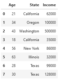
Before we can train a model on this data, we need to do something about the "State" column. While its current format is great for human readability, a machine learning model is going to have trouble understanding it, as models like numbers.
A first attempt at this might involve simply assigning the number 1–6 to the six different states we have above. While a good idea for ordinal variables, this won’t work well for our nominal variable, as it implies an ordering in the data which does not exist.
The most common conversion technique for nominal variables is known as one-hot encoding. One-hot encoding is the process of converting one column with different categorical values into multiple columns (one for each distinct categorical value), and a binary integer for each row indicating whether or not it fits into that column [3].
So, instead of having one column called "State" , we would reorganize our data to have the columns "is_state_California" , "is_state_Oregon" , and so on for each unique state present in the data. Then, the rows which initially had a value of "California" for the "State" column would have a value of 1 in the "is_state_California" column, and a value of 0 in all the other columns.
Now for the important part: how do we actually implement this in Pandas? Having done all the conceptual work to get to this point, you’ll be pleased to learn the code itself is actually fairly straightforward: Pandas has a function called get_dummies which does all the work of one-hot encoding for us [4]. Assuming our DataFrame above is called my_df, we would do the following:
pd.get_dummies(my_df, columns=["State"], prefix='is_state')

And there you have it! Your data is now in a format far more conducive to training a machine learning model.
Merging DataFrames Together
If you’ve been in the realm of data science for any meaningful length of time, you’re well aware that data in its initial form is always ugly. Always. Without exception. If you’re just entering into the field, this is a reality you’ll become familiar with very soon.
Accordingly, a large part of a data scientist’s job involves combining together data from disparate locations and cleaning up missing values. One of the most important — and unfortunately also one of the most complex — methods for combining data is via a merge.
In principle, the idea behind merging actually isn’t too bad: it simply provides a way to combine the data from two different DataFrames which have different information, but at least one column with matching values. However, the implementation can get confusing because there are many different types of merges (also known as joins).
As always, let’s look at an example. Let’s start with the similar DataFrame as above, except this time it also has names and is called left_df (you’ll see why in a moment):

We also have a second DataFrame called right_df, which contains additional information about college degrees for various people, some of whom are the same as in left_df:
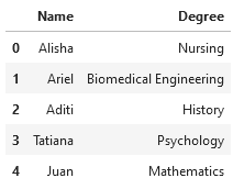
We’re interested in adding a person’s degree as a feature for our model, so we decide to merge these two DataFrames together. When we merge, we need to specify a few different things:
- The left DataFrame
- The right DataFrame
- The column(s) we want to merge on
- What type of join we want: inner, left, right, or outer
The final specification above is where things get confusing, so let’s walk through each of them in detail.
An inner join will merge together the two DataFrames so that only rows which have a match in both DataFrames appear in the output DataFrame. For example, with our above two DataFrames, this would look like the following:
left_df.merge(right_df, on='Name', how='inner')
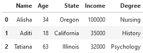
Only Alisha, Aditi, and Tatiana appear in both DataFrames, and as such only their rows are part of the output when merging via an inner join. We can also see that the "Degree" column is now present, illustrating why we merged in the first place.
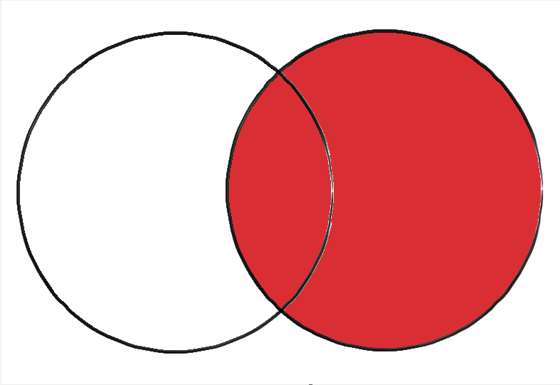
Below is a graphic depicting an inner join visually. The left circle can be though of as left_df, and the right as right_df.

A left join includes all of the rows in the left DataFrame, even if they don’t have a match in the right DataFrame. For those that aren’t present in the right DataFrame (and thus don’t have a value in the new column, in this case "Degree"), Pandas fills in a null value. Later in this article, we’ll see how we can deal with such values.
Importantly, this type of merge does not include values in the right DataFrame that don’t have a match in the left. Let’s take a look at our example:
left_df.merge(right_df, on='Name', how='left')
We can see that all the people from left_df are present, even if they didn’t have a match in right_df. On the other hand, Ariel and Juan, who are only in right_df, are not in the output DataFrame.
Here’s a graphical depiction of a left join:

A right join is almost exactly the same as a left join, except this time it includes all values from the right DataFrame rather than the left one, similarly filling in mismatches with null values:
left_df.merge(right_df, on='Name', how='right')

This time it’s Ted, Aaron, Lee, Abdul, and Khadija missing from the output, as they are not present in right_df. Here’s a right join shown graphically:
The final type of merge is done via an outer join. As you might have guessed, this type of join includes all the rows across both DataFrames, filling in all of the missing values with nulls. With our data, this looks as follows:
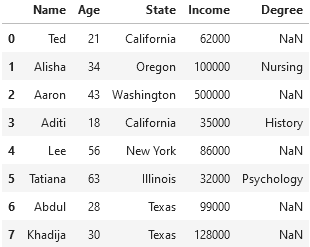
left_df.merge(right_df, on='Name', how='outer')

We can see how Pandas fills in NaN for the "Degree" values of Ted, Aaron, Lee, Abdul, and Khadija, as they aren’t present in right_df and thus don’t have corresponding data for that column. Similarly, Ariel and Juan have NaN values for "State" and "Income", as they don’t exist in left_df.
Here’s a graphical depiction of an outer join:

And with that, you should be ready to merge out in the wild.
Let’s move on to our second underappreciated skill.
Concatenating DataFrames Together
After the maze of possibilities within merge, you’ll be pleased to learn that concatenation is fairly straightforward. It also involves combining two DataFrames, except instead of connecting columns based on a common label, it’s more like just stacking two DataFrames together. Additionally, it is an operation that can also be performed on more than two DataFrames at a time.
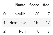
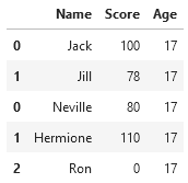
The most basic example of concatenation involves two DataFrames whose columns are identical [5]. For example, say we have the following two DataFrames, called top_df and bottom_df, respectively:


We can concatenate them as follows:
pd.concat([top_df, bottom_df])

A couple important notes about the above:
- Unlike
merge, which we often call directly on the DataFrame object (e.g.top_df.merge(bottom_df), we callconcatusingpd.concat. - The DataFrames we are concatenating are passed in as one argument within a list, not two (or more) separate arguments.
We can also concatenate DataFrames which aren’t exact matches. For example, say we add another column to our bottom_df:
Then, the same concatenation gives us the following output DataFrame:

It works, but it isn’t ideal, as we’ll eventually need to do something about those pesky null values as well as convert the floats back to integers (see the next section).
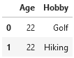
Finally, concatenation also works horizontally. To see this, we’ll add one more DataFrame to our arsenal, called more_df:
Then, we get the following:
pd.concat([top_df, more_df], axis=1)
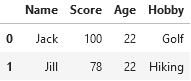
The additional argument axis=1 tells Pandas that we want to combine horizontally (by column); if we omit this argument, it defaults to axis=0, which combines vertically (by row).
Note that horizontal concatenation is different from merging two DataFrames because it does not choose a common column to join together to DataFrames; it basically just sticks two disparate DataFrames together without worrying about the presence of common labels.
And that’s all there is to it.
Bonus Skill: Fill and Replace
You may have noticed that when we collect data from different places into one location, we often end up with annoying null values or mistyped data entries. Let’s take a look at how we can fix these issues. As an example, we’ll use one of the above DataFrames, this time calling it faulty_df:
Null values represent data we don’t have; in many cases, we want to fill these values in so that we can perform our analyses without running into errors. There are many techniques for filling in missing data, but we’ll just pick a simple one for this example: using the average value — in this case 17.
The easiest way to achieve this in Pandas is via the fill_na function:
faulty_df = faulty_df.fillna(17)
faulty_df

Then, we can convert these floats back to the desired type — integers — via the astype function:
faulty_df['Age'] = faulty_df['Age'].astype('int')
faulty_df
And there you have it — a simple way to deal with the few broken DataFrame entries you may get after merging and concatenating.
Recap and Final Thoughts
As a data scientist, it’s extremely important to be comfortable collecting, organizing, cleaning, and restructuring data to suit your analysis needs. By mastering the skills above, you’ll get one step closer to that ideal.
Here’s a cheat sheet for future reference:
- Categorical data doesn’t vibe with ML models. Learn one-hot encoding.
- Data you need is often scattered. Get good at merging it together.
- Similar data sets belong together. Help them unite via concatenation.
Best of luck in your data manipulation endeavors.
One-hot encode, merge, and concatenate: say hello to useful data transformations and funky data combinations.
This is the third article in my Next-Level Series. Be sure to check out the first two: 3 Underappreciated Skills to Make You a Next-Level Data Scientist and 3 Underappreciated Skills to Make You a Next-Level Python Programmer.
It’s no secret that Pandas is a difficult module to learn. It can be confusing and overwhelming — especially for newer programmers. However, it is also incredibly important if you’re going to be a data scientist.
For this reason, even data science educational programs are starting to shift toward a model that emphasizes learning Pandas more than before. When I first learned data science (about 4 years ago), my course at UC Berkeley used an in-house module called datascience [1], built on top of Pandas but quite different in functionality.
But courses are starting to change. Recently, UC San Diego came out with a module designed to prepare students for the transition to full-blown Pandas — accordingly, they call it babypandas [2].
Both individuals and institutions are beginning to realize that understanding Pandas is a must for modern data science, and they are shaping their educational aspirations around that premise.
If you’re reading this, it’s likely you’re one of them. Allow me to help you on your way.
Let’s take a look at 3 underappreciated skills that’ll help you become a next-level Pandas user.
One-Hot Encoding for Categorical Variables
To properly understand this skill, we need to do a quick review of the different types of variables in a statistical context. The two overarching types of variables are quantitative and qualitative (categorical), which can be further sub-divided into the following groups:
- Discrete (Quantitative): this is a numerical value, but one which can be counted exactly. For example, if your variable is a city’s population, it would be a discrete variable. Why? Well, it’s clearly a number on which you can perform various arithmetic calculations, but at the same time it wouldn’t make sense to say the population of a city is 786.5 people. It must be an exact number.
- Continuous (Quantitative): this is again a numerical value, but one which is measured, and thus can never be determined exactly. An example is height. While we might measure it to the nearest centimeter or millimeter because of the available tools, in theory we could go as deep as we wanted with extremely granular measurements (micrometers, nanometers, picometers, and so on).
- Ordinal (Categorical): this is a qualitative variable — that is, it is not a number on which it makes sense to perform arithmetic. Such a variable can take on any value within a finite number of ordered categories. For example, you might have a variable “spice level” with potential values of “mild,” “medium,” or “hot.”
- Nominal (Categorical): this is similar to an ordinal variable, except the categories have no clear hierarchy to them. A common example of a nominal variable is color.
One note about the above definitions: ordinal and nominal variables can often still be numbers; the distinction is that it doesn’t make sense to perform arithmetic on these numbers. For instance, a geographical zip code is a nominal variable, not a quantitative one, because it makes no sense to take the sum or difference (or product, quotient, etc.) of two zip codes.
Now that we’ve reviewed the above, we can address the chief problem: computers like quantitative data, but the data we have available is often qualitative. Particularly in the context of building predictive models, we need a way to represent categorical data in a way that makes sense to the model. This is best seen via example.
Imagine we have a data set with three columns: "Age" , "State" , and "Income" . We want to build a model which uses a person’s state of residence and their age to predict their income. A subset of our data set might look something like the following:
Before we can train a model on this data, we need to do something about the "State" column. While its current format is great for human readability, a machine learning model is going to have trouble understanding it, as models like numbers.
A first attempt at this might involve simply assigning the number 1–6 to the six different states we have above. While a good idea for ordinal variables, this won’t work well for our nominal variable, as it implies an ordering in the data which does not exist.
The most common conversion technique for nominal variables is known as one-hot encoding. One-hot encoding is the process of converting one column with different categorical values into multiple columns (one for each distinct categorical value), and a binary integer for each row indicating whether or not it fits into that column [3].
So, instead of having one column called "State" , we would reorganize our data to have the columns "is_state_California" , "is_state_Oregon" , and so on for each unique state present in the data. Then, the rows which initially had a value of "California" for the "State" column would have a value of 1 in the "is_state_California" column, and a value of 0 in all the other columns.
Now for the important part: how do we actually implement this in Pandas? Having done all the conceptual work to get to this point, you’ll be pleased to learn the code itself is actually fairly straightforward: Pandas has a function called get_dummies which does all the work of one-hot encoding for us [4]. Assuming our DataFrame above is called my_df, we would do the following:
pd.get_dummies(my_df, columns=["State"], prefix='is_state')
And there you have it! Your data is now in a format far more conducive to training a machine learning model.
Merging DataFrames Together
If you’ve been in the realm of data science for any meaningful length of time, you’re well aware that data in its initial form is always ugly. Always. Without exception. If you’re just entering into the field, this is a reality you’ll become familiar with very soon.
Accordingly, a large part of a data scientist’s job involves combining together data from disparate locations and cleaning up missing values. One of the most important — and unfortunately also one of the most complex — methods for combining data is via a merge.
In principle, the idea behind merging actually isn’t too bad: it simply provides a way to combine the data from two different DataFrames which have different information, but at least one column with matching values. However, the implementation can get confusing because there are many different types of merges (also known as joins).
As always, let’s look at an example. Let’s start with the similar DataFrame as above, except this time it also has names and is called left_df (you’ll see why in a moment):
We also have a second DataFrame called right_df, which contains additional information about college degrees for various people, some of whom are the same as in left_df:
We’re interested in adding a person’s degree as a feature for our model, so we decide to merge these two DataFrames together. When we merge, we need to specify a few different things:
- The left DataFrame
- The right DataFrame
- The column(s) we want to merge on
- What type of join we want: inner, left, right, or outer
The final specification above is where things get confusing, so let’s walk through each of them in detail.
An inner join will merge together the two DataFrames so that only rows which have a match in both DataFrames appear in the output DataFrame. For example, with our above two DataFrames, this would look like the following:
left_df.merge(right_df, on='Name', how='inner')
Only Alisha, Aditi, and Tatiana appear in both DataFrames, and as such only their rows are part of the output when merging via an inner join. We can also see that the "Degree" column is now present, illustrating why we merged in the first place.
Below is a graphic depicting an inner join visually. The left circle can be though of as left_df, and the right as right_df.
A left join includes all of the rows in the left DataFrame, even if they don’t have a match in the right DataFrame. For those that aren’t present in the right DataFrame (and thus don’t have a value in the new column, in this case "Degree"), Pandas fills in a null value. Later in this article, we’ll see how we can deal with such values.
Importantly, this type of merge does not include values in the right DataFrame that don’t have a match in the left. Let’s take a look at our example:
left_df.merge(right_df, on='Name', how='left')
We can see that all the people from left_df are present, even if they didn’t have a match in right_df. On the other hand, Ariel and Juan, who are only in right_df, are not in the output DataFrame.
Here’s a graphical depiction of a left join:
A right join is almost exactly the same as a left join, except this time it includes all values from the right DataFrame rather than the left one, similarly filling in mismatches with null values:
left_df.merge(right_df, on='Name', how='right')
This time it’s Ted, Aaron, Lee, Abdul, and Khadija missing from the output, as they are not present in right_df. Here’s a right join shown graphically:
The final type of merge is done via an outer join. As you might have guessed, this type of join includes all the rows across both DataFrames, filling in all of the missing values with nulls. With our data, this looks as follows:
left_df.merge(right_df, on='Name', how='outer')
We can see how Pandas fills in NaN for the "Degree" values of Ted, Aaron, Lee, Abdul, and Khadija, as they aren’t present in right_df and thus don’t have corresponding data for that column. Similarly, Ariel and Juan have NaN values for "State" and "Income", as they don’t exist in left_df.
Here’s a graphical depiction of an outer join:
And with that, you should be ready to merge out in the wild.
Let’s move on to our second underappreciated skill.
Concatenating DataFrames Together
After the maze of possibilities within merge, you’ll be pleased to learn that concatenation is fairly straightforward. It also involves combining two DataFrames, except instead of connecting columns based on a common label, it’s more like just stacking two DataFrames together. Additionally, it is an operation that can also be performed on more than two DataFrames at a time.
The most basic example of concatenation involves two DataFrames whose columns are identical [5]. For example, say we have the following two DataFrames, called top_df and bottom_df, respectively:
We can concatenate them as follows:
pd.concat([top_df, bottom_df])
A couple important notes about the above:
- Unlike
merge, which we often call directly on the DataFrame object (e.g.top_df.merge(bottom_df), we callconcatusingpd.concat. - The DataFrames we are concatenating are passed in as one argument within a list, not two (or more) separate arguments.
We can also concatenate DataFrames which aren’t exact matches. For example, say we add another column to our bottom_df:
Then, the same concatenation gives us the following output DataFrame:
It works, but it isn’t ideal, as we’ll eventually need to do something about those pesky null values as well as convert the floats back to integers (see the next section).
Finally, concatenation also works horizontally. To see this, we’ll add one more DataFrame to our arsenal, called more_df:
Then, we get the following:
pd.concat([top_df, more_df], axis=1)
The additional argument axis=1 tells Pandas that we want to combine horizontally (by column); if we omit this argument, it defaults to axis=0, which combines vertically (by row).
Note that horizontal concatenation is different from merging two DataFrames because it does not choose a common column to join together to DataFrames; it basically just sticks two disparate DataFrames together without worrying about the presence of common labels.
And that’s all there is to it.
Bonus Skill: Fill and Replace
You may have noticed that when we collect data from different places into one location, we often end up with annoying null values or mistyped data entries. Let’s take a look at how we can fix these issues. As an example, we’ll use one of the above DataFrames, this time calling it faulty_df:
Null values represent data we don’t have; in many cases, we want to fill these values in so that we can perform our analyses without running into errors. There are many techniques for filling in missing data, but we’ll just pick a simple one for this example: using the average value — in this case 17.
The easiest way to achieve this in Pandas is via the fill_na function:
faulty_df = faulty_df.fillna(17)
faulty_df
Then, we can convert these floats back to the desired type — integers — via the astype function:
faulty_df['Age'] = faulty_df['Age'].astype('int')
faulty_df
And there you have it — a simple way to deal with the few broken DataFrame entries you may get after merging and concatenating.
Recap and Final Thoughts
As a data scientist, it’s extremely important to be comfortable collecting, organizing, cleaning, and restructuring data to suit your analysis needs. By mastering the skills above, you’ll get one step closer to that ideal.
Here’s a cheat sheet for future reference:
- Categorical data doesn’t vibe with ML models. Learn one-hot encoding.
- Data you need is often scattered. Get good at merging it together.
- Similar data sets belong together. Help them unite via concatenation.
Best of luck in your data manipulation endeavors.
Denial of responsibility! Techno Blender is an automatic aggregator of the all world’s media. In each content, the hyperlink to the primary source is specified. All trademarks belong to their rightful owners, all materials to their authors. If you are the owner of the content and do not want us to publish your materials, please contact us by email – [email protected]. The content will be deleted within 24 hours.