
5 Most Well-Known CNN Architectures Visualized | by Albers Uzila | Aug, 2022
Deep Learning
Understanding CNN from the ground up
Table of Contents· Fully Connected Layer and Activation Function· Convolution and Pooling Layer· Normalization Layer
∘ Local Response Normalization
∘ Batch Normalization· 5 Most Well-Known CNN Architectures Visualized
∘ LeNet-5
∘ AlexNet
∘ VGG-16
∘ Inception-v1
∘ ResNet-50· Wrapping Up
The introduction of LeNet in 1990 by Yann LeCun sparks the possibility of deep neural networks in practice. However, limited computation capability and memory capacity made the algorithm difficult to implement until about 2010.
While LeNet is the one that starts the era of Convolutional Neural Networks (CNN), AlexNet — invented by Alex Krizhevsky and others in 2012 — is the one that starts the era of CNN used for ImageNet classification.
AlexNet is the first evidence that CNN can perform well on this historically complex ImageNet dataset and it performs so well that leads society into a competition of developing CNNs: from VGG, Inception, ResNet, to EfficientNet.
Most of these architectures follow the same recipe: combos of convolution layers and pooling layers followed by fully connected layers, with some layers having an activation function and/or normalization step. You will learn all these mumbo jumbos first, so all architectures can be understood easily afterward.
Note: If you want the editable version of the architectures explained in this story, please visit my gumroad page below.
With this template, you might want to edit existing architectures for your own presentations, education, or research purposes, or you might want to use our beautiful legend to build other amazing deep learning architectures but don’t want to start from scratch. It’s FREE (or pay what you want)!
Let’s go back in time. In 1958, Frank Rosenblatt introduced the first perceptron, an electronic device that was constructed by biological principles and showed an ability to learn. The perceptron was intended to be a machine, rather than a program, and one of its first implementations was designed for image recognition.
The machine highly resembles a modern perceptron. In the modern sense, the perceptron is an algorithm for learning a binary classifier as shown below. Perceptron gives a linear decision boundary between two classes utilizing a step function that depends on the weighted sum of data.
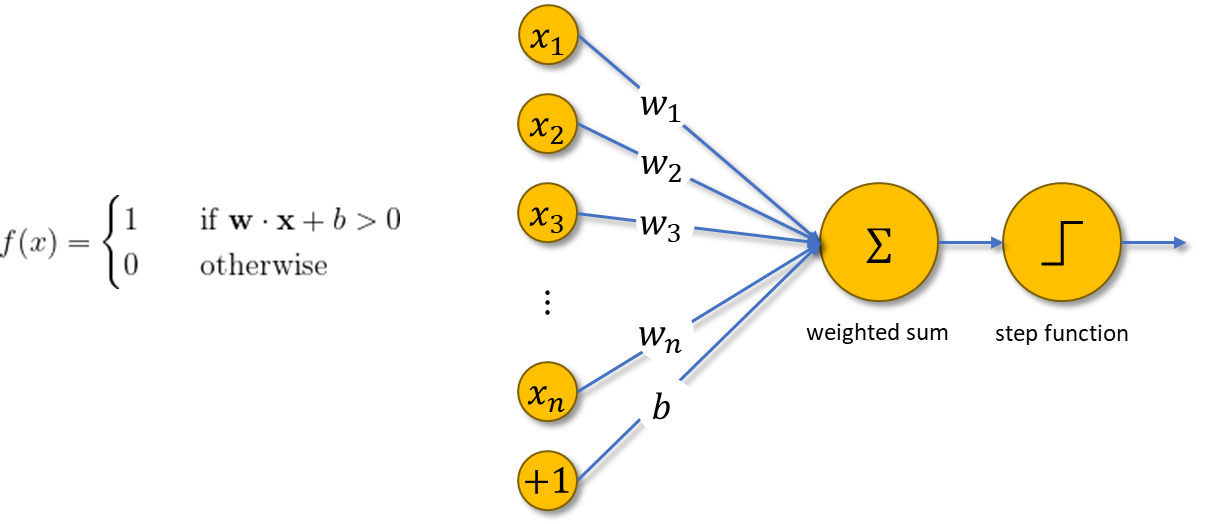
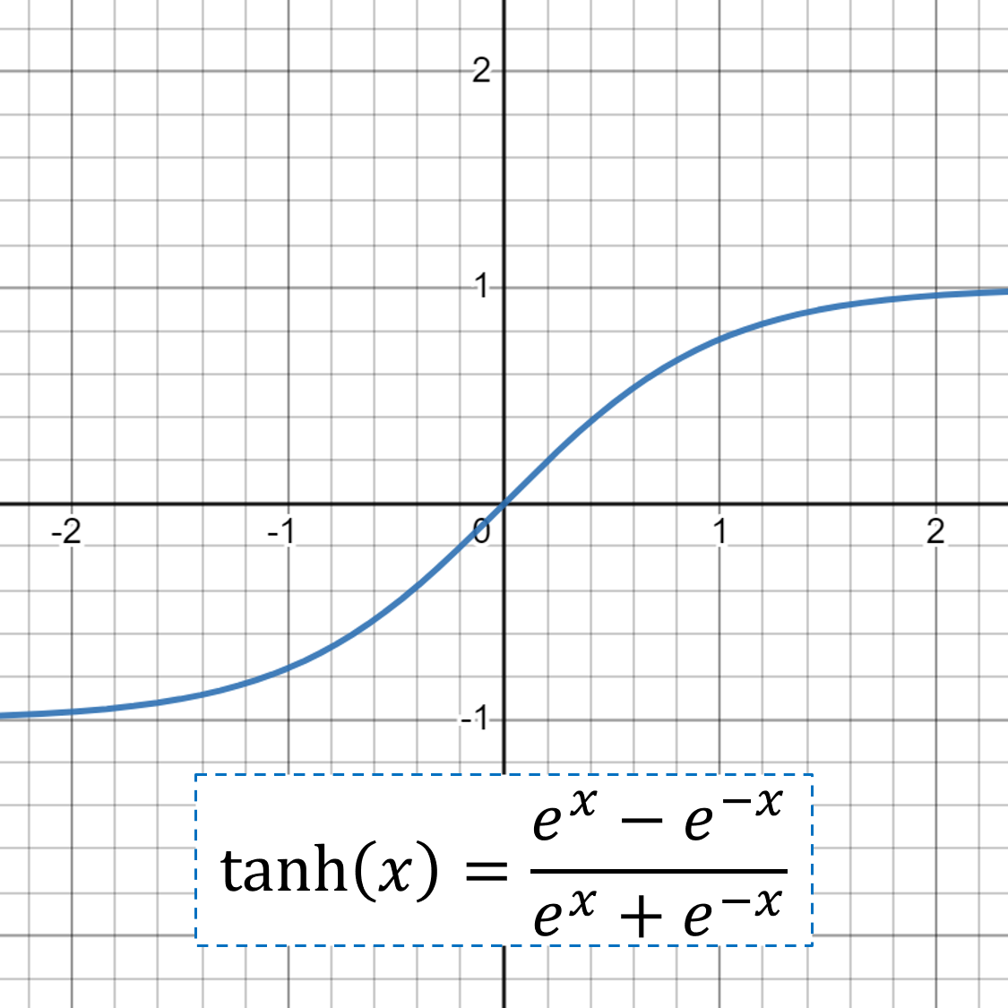
The step function in a perceptron is an example of an activation function; it activates whether the state of the perceptron is on (1) or off (0). Nowadays, there are many kinds of activation functions, most of which can be used to introduce nonlinearities to perceptrons. Some common activation functions besides the step function are:


The perceptron is called the logistic regression model if the activation function is sigmoid.
There’s also another activation function worth mentioning that is used when dealing with multiclass classification tasks: softmax. Consider a task with K classes, then softmax is expressed by

Softmax gives the predicted probability that class i will be selected by the model. The model with a softmax activation function will pick the class with the highest probability as the final prediction.
Consider a perceptron with an arbitrary activation function g. You can stack as many perceptrons as you like on top of each other into a single layer, and you can connect the outputs of a layer to another layer. The result is what we call a Multi-Layer Perceptron (MLP).

In a vectorized formulation, MLP with L layers is expressed as follows.

MLP is also called a dense neural network since it resembles how the brain works. Each unit circle in the last image above is called a neuron. In the world of neural networks, MLP layers are also called fully connected layers since every neuron in a layer is connected to all neurons in the next layer.
Fully connected layers are useful when it’s difficult to find a meaningful way to extract features from data, e.g. tabular data. When it comes to image data, CNN is arguably the most well-known family of neural networks to have. For image data, neural networks use the RGB channel of an image to work with.

CNN allows the neural network to reuse parameters across different spatial locations of an image. Various choices of filters (also called kernels) could achieve different image operations: identity, edge detection, blur, sharpening, etc. The idea of CNN is to discover some interesting features of the image by introducing random matrices as a convolution operator.
After the image has been convolved with kernels, you’re left with what’s known as a feature map. You can convolve your feature maps again and again to extract features, however, this turns out to be incredibly computationally expensive. Instead, you can reduce the size of your feature maps using the pooling layer.
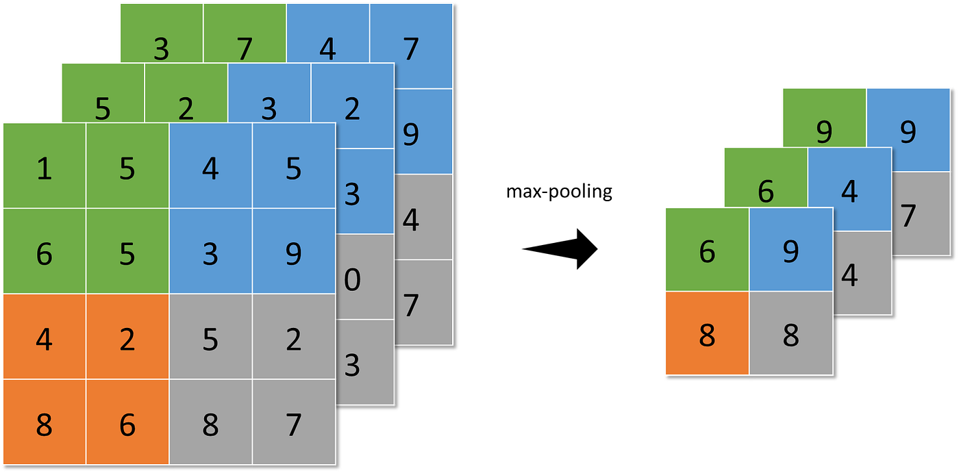
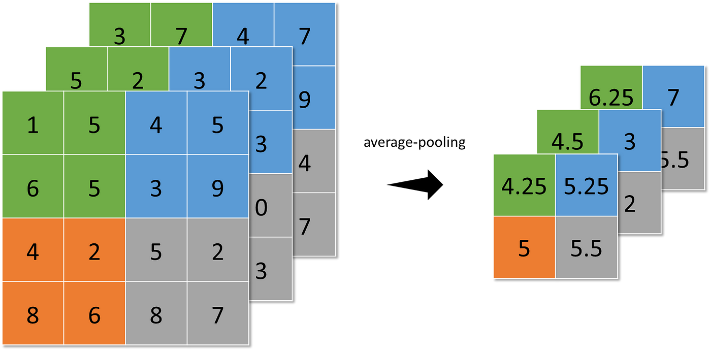
The pooling layer represents small regions of a feature map by a single pixel. Some different strategies can be considered:
- max-pooling (the highest value is selected from the N×N patches of the feature maps),
- average-pooling (sums up over N×N patches of the feature maps from the previous layer and selects the average value), and
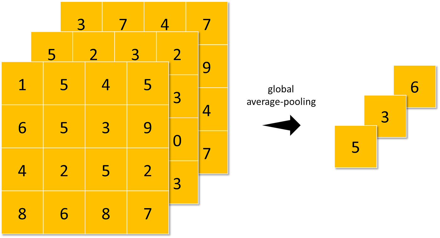
- global-average-pooling (similar to average-pooling but instead of using N×N patches of the feature maps, it uses all feature maps area at once).
Pooling makes the neural network invariant to small transformations, distortions, and translations in the input image. A small distortion in the input will not change the outcome of pooling since you take the maximum/average value in a local neighborhood.
Local Response Normalization
In his AlexNet paper, Alex Krizhevsky and others introduced Local Response Normalization (LRN), a scheme to aid the generalization capability of AlexNet.
LRN implements the idea of lateral inhibition, a concept in neurobiology that refers to the phenomenon of an excited neuron inhibiting its neighbors: this leads to a peak in the form of a local maximum, creating contrast in that area and increasing sensory perception.
Given aᵢ the activity of a neuron computed by applying kernel i and then applying the activation function, the response-normalized activity bᵢ is given by the expression

where the sum runs over n “adjacent” kernel maps at the same spatial position, and N is the total number of kernels in the layer. The constants k, n, α, and β are hyperparameters.
To be concrete, let (k, n, α, β) = (0, 2, 1, 1). After being applied to LRN, we will calculate the value of the top left pixel (colored lightest green below).

Here’s the calculation.

Batch Normalization
Another breakthrough in the optimization of deep neural networks is Batch Normalization (BN). It addresses the problem called internal covariate shift:
The changes in parameters of the previous neural network layers change the input/covariate of the current layer. This change could be dramatic as it may shift the distribution of inputs. And a layer is barely useful if its input change.
Let m be the batch size during training. For every batch, BN formally follows the steps:

where

This way, BN helps accelerate deep neural network training. The network converges faster and shows better regularization during training, which has an impact on the overall accuracy.
You’ve learned the following:
- Convolution Layer
- Pooling Layer
- Normalization Layer
- Fully Connected Layer
- Activation Function
Now, we’re ready to introduce and visualize 5 CNN architectures:
They will be built on top of the layers and functions you learned. So, to simplify things, we will cut out some information such as the number of filters, stride, padding, and dropout for regularization. You will use the following legend to aid you.

Note: This part of the story is largely inspired by the following story by Raimi Karim. Make sure you check it out!
Let’s begin, shall we?
This starts it all. Excluding pooling, LeNet-5 consists of 5 layers:
- 2 convolution layers with kernel size 5×5, followed by
- 3 fully connected layers.
Each convolution layer is followed by a 2×2 average-pooling, and every layer has tanh activation function except the last (which has softmax).
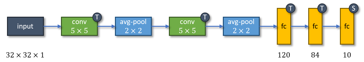
LeNet-5 has 60,000 parameters. The network is trained on greyscale 32×32 digit images and tries to recognize them as one of the ten digits (0 to 9).
AlexNet introduces the ReLU activation function and LRN into the mix. ReLU becomes so popular that almost all CNN architectures developed after AlexNet used ReLU in their hidden layers, abandoning the use of tanh activation function in LeNet-5.

The network consists of 8 layers:
- 5 convolution layers with non-increasing kernel sizes, followed by
- 3 fully connected layers.
The last layer uses the softmax activation function, and all others use ReLU. LRN is applied on the first and second convolution layers after applying ReLU. The first, second, and fifth convolution layers are followed by a 3×3 max pooling.
With the advancement of modern hardware, AlexNet can be trained with a whopping 60 million parameters and becomes the winner of the ImageNet competition in 2012. ImageNet has become a benchmark dataset in developing CNN architectures and a subset of it (ILSVRC) consists of various images with 1000 classes. Default AlexNet accepts colored images with dimensions 224×224.
Researchers investigated the effect of the CNN depth on its accuracy in the large-scale image recognition setting. By pushing the depth to 11–19 layers, VGG families are born: VGG-11, VGG-13, VGG-16, and VGG-19. A version of VGG-11 with LRN was also investigated but LRN doesn’t improve the performance. Hence, all other VGGs are implemented without LRN.

This story focuses on VGG-16, a deep CNN architecture with, well, 16 layers:
- 13 convolution layers with kernel size 3×3, followed by
- 3 fully connected layers.
VGG-16 is one of the biggest networks that has 138 million parameters. Just like AlexNet, the last layer is equipped with a softmax activation function and all others are equipped with ReLU. The 2nd, 4th, 7th, 10th, and 13th convolution layers are followed by a 2×2 max-pooling. Default VGG-16 accepts colored images with dimensions 224×224 and outputs one of the 1000 classes.
Going deeper has a caveat: exploding/vanishing gradients:
- The exploding gradient is a problem when large error gradients accumulate and result in unstable weight updates during training.
- The vanishing gradient is a problem when the partial derivative of the loss function approaches a value close to zero and the network couldn’t train.

Inception-v1 tackles this issue by adding two auxiliary classifiers connected to intermediate layers, with the hope to increase the gradient signal that gets propagated back. During training, their loss gets added to the total loss of the network with a 0.3 discount weight. At inference time, these auxiliary networks are discarded.
Inception-v1 introduces the inception module, four series of one or two convolution and max-pool layers stacked in parallel and concatenated at the end. The inception module aims to approximate an optimal local sparse structure in a CNN by allowing the use of multiple types of kernel sizes, instead of being restricted to single kernel size.
Inception-v1 has fewer parameters than AlexNet and VGG-16, a mere 7 million, even though it consists of 22 layers:
- 3 convolution layers with 7×7, 1×1, and 3×3 kernel sizes, followed by
- 18 layers that consist of 9 inception modules where each has 2 layers of convolution/max-pooling, followed by
- 1 fully connected layer.
The last layer of the main classifier and the two auxiliary classifiers are equipped with a softmax activation function and all others are equipped with ReLU. The 1st and 3rd convolution layers, also the 2nd and 7th inception modules are followed by a 3×3 max-pooling. The last inception module is followed by a 7×7 average-pooling. LRN is applied after the 1st max-pooling and the 3rd convolution layer.
Auxiliary classifiers are branched out after the 3rd and 6th inception modules, each starts with a 5×5 average-pooling and is then followed by 3 layers:
- 1 convolution layer with 1×1 kernel size, and
- 2 fully connected layers.
Default Inception-v1 accepts colored images with dimensions 224×224 and outputs one of the 1000 classes.
When deeper networks can start converging, a degradation problem has been exposed: with the network depth increasing, accuracy gets saturated and then degrades rapidly.
Unexpectedly, such degradation is not caused by overfitting (usually indicated by lower training error and higher testing error) since adding more layers to a suitably deep network leads to higher training error.

The degradation problem is addressed by introducing bottleneck residual blocks. There are 2 kinds of residual blocks:
- Identity block: consists of 3 convolution layers with 1×1, 3×3, and 1×1 kernel sizes, all of which are equipped with BN. ReLU activation function is applied to the first two layers, while the input of the identity block is added to the last layer before applying ReLU.
- Convolution block: same as identity block, but the input of the convolution block is first passed through a convolution layer with 1×1 kernel size and BN before being added to the last convolution layer of the main series.
Notice that both residual blocks have 3 layers. In total, ResNet-50 has 26 million parameters and 50 layers:
- 1 convolution layer with BN then ReLU is applied, followed by
- 9 layers that consist of 1 convolution block and 2 identity blocks, followed by
- 12 layers that consist of 1 convolution block and 3 identity blocks, followed by
- 18 layers that consist of 1 convolution block and 5 identity blocks, followed by
- 9 layers that consist of 1 convolution block and 2 identity blocks, followed by
- 1 fully connected layer with softmax.
The first convolution layer is followed by a 3×3 max-pooling and the last identity block is followed by a global-average-pooling. Default ResNet-50 accepts colored images with dimensions 224×224 and outputs one of the 1000 classes.
Here’s a summary of all architectures.

Deep Learning
Understanding CNN from the ground up
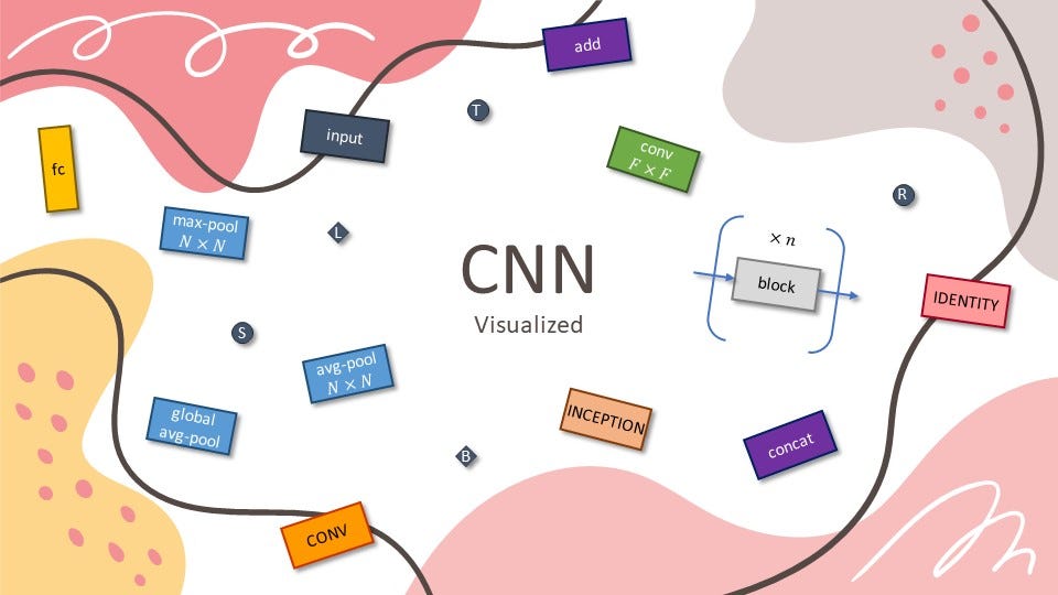
Table of Contents· Fully Connected Layer and Activation Function· Convolution and Pooling Layer· Normalization Layer
∘ Local Response Normalization
∘ Batch Normalization· 5 Most Well-Known CNN Architectures Visualized
∘ LeNet-5
∘ AlexNet
∘ VGG-16
∘ Inception-v1
∘ ResNet-50· Wrapping Up
The introduction of LeNet in 1990 by Yann LeCun sparks the possibility of deep neural networks in practice. However, limited computation capability and memory capacity made the algorithm difficult to implement until about 2010.
While LeNet is the one that starts the era of Convolutional Neural Networks (CNN), AlexNet — invented by Alex Krizhevsky and others in 2012 — is the one that starts the era of CNN used for ImageNet classification.
AlexNet is the first evidence that CNN can perform well on this historically complex ImageNet dataset and it performs so well that leads society into a competition of developing CNNs: from VGG, Inception, ResNet, to EfficientNet.
Most of these architectures follow the same recipe: combos of convolution layers and pooling layers followed by fully connected layers, with some layers having an activation function and/or normalization step. You will learn all these mumbo jumbos first, so all architectures can be understood easily afterward.
Note: If you want the editable version of the architectures explained in this story, please visit my gumroad page below.
With this template, you might want to edit existing architectures for your own presentations, education, or research purposes, or you might want to use our beautiful legend to build other amazing deep learning architectures but don’t want to start from scratch. It’s FREE (or pay what you want)!
Let’s go back in time. In 1958, Frank Rosenblatt introduced the first perceptron, an electronic device that was constructed by biological principles and showed an ability to learn. The perceptron was intended to be a machine, rather than a program, and one of its first implementations was designed for image recognition.
The machine highly resembles a modern perceptron. In the modern sense, the perceptron is an algorithm for learning a binary classifier as shown below. Perceptron gives a linear decision boundary between two classes utilizing a step function that depends on the weighted sum of data.
The step function in a perceptron is an example of an activation function; it activates whether the state of the perceptron is on (1) or off (0). Nowadays, there are many kinds of activation functions, most of which can be used to introduce nonlinearities to perceptrons. Some common activation functions besides the step function are:
The perceptron is called the logistic regression model if the activation function is sigmoid.
There’s also another activation function worth mentioning that is used when dealing with multiclass classification tasks: softmax. Consider a task with K classes, then softmax is expressed by
Softmax gives the predicted probability that class i will be selected by the model. The model with a softmax activation function will pick the class with the highest probability as the final prediction.
Consider a perceptron with an arbitrary activation function g. You can stack as many perceptrons as you like on top of each other into a single layer, and you can connect the outputs of a layer to another layer. The result is what we call a Multi-Layer Perceptron (MLP).
In a vectorized formulation, MLP with L layers is expressed as follows.
MLP is also called a dense neural network since it resembles how the brain works. Each unit circle in the last image above is called a neuron. In the world of neural networks, MLP layers are also called fully connected layers since every neuron in a layer is connected to all neurons in the next layer.
Fully connected layers are useful when it’s difficult to find a meaningful way to extract features from data, e.g. tabular data. When it comes to image data, CNN is arguably the most well-known family of neural networks to have. For image data, neural networks use the RGB channel of an image to work with.
CNN allows the neural network to reuse parameters across different spatial locations of an image. Various choices of filters (also called kernels) could achieve different image operations: identity, edge detection, blur, sharpening, etc. The idea of CNN is to discover some interesting features of the image by introducing random matrices as a convolution operator.
After the image has been convolved with kernels, you’re left with what’s known as a feature map. You can convolve your feature maps again and again to extract features, however, this turns out to be incredibly computationally expensive. Instead, you can reduce the size of your feature maps using the pooling layer.
The pooling layer represents small regions of a feature map by a single pixel. Some different strategies can be considered:
- max-pooling (the highest value is selected from the N×N patches of the feature maps),
- average-pooling (sums up over N×N patches of the feature maps from the previous layer and selects the average value), and
- global-average-pooling (similar to average-pooling but instead of using N×N patches of the feature maps, it uses all feature maps area at once).
Pooling makes the neural network invariant to small transformations, distortions, and translations in the input image. A small distortion in the input will not change the outcome of pooling since you take the maximum/average value in a local neighborhood.
Local Response Normalization
In his AlexNet paper, Alex Krizhevsky and others introduced Local Response Normalization (LRN), a scheme to aid the generalization capability of AlexNet.
LRN implements the idea of lateral inhibition, a concept in neurobiology that refers to the phenomenon of an excited neuron inhibiting its neighbors: this leads to a peak in the form of a local maximum, creating contrast in that area and increasing sensory perception.
Given aᵢ the activity of a neuron computed by applying kernel i and then applying the activation function, the response-normalized activity bᵢ is given by the expression
where the sum runs over n “adjacent” kernel maps at the same spatial position, and N is the total number of kernels in the layer. The constants k, n, α, and β are hyperparameters.
To be concrete, let (k, n, α, β) = (0, 2, 1, 1). After being applied to LRN, we will calculate the value of the top left pixel (colored lightest green below).
Here’s the calculation.
Batch Normalization
Another breakthrough in the optimization of deep neural networks is Batch Normalization (BN). It addresses the problem called internal covariate shift:
The changes in parameters of the previous neural network layers change the input/covariate of the current layer. This change could be dramatic as it may shift the distribution of inputs. And a layer is barely useful if its input change.
Let m be the batch size during training. For every batch, BN formally follows the steps:
where
This way, BN helps accelerate deep neural network training. The network converges faster and shows better regularization during training, which has an impact on the overall accuracy.
You’ve learned the following:
- Convolution Layer
- Pooling Layer
- Normalization Layer
- Fully Connected Layer
- Activation Function
Now, we’re ready to introduce and visualize 5 CNN architectures:
They will be built on top of the layers and functions you learned. So, to simplify things, we will cut out some information such as the number of filters, stride, padding, and dropout for regularization. You will use the following legend to aid you.
Note: This part of the story is largely inspired by the following story by Raimi Karim. Make sure you check it out!
Let’s begin, shall we?
This starts it all. Excluding pooling, LeNet-5 consists of 5 layers:
- 2 convolution layers with kernel size 5×5, followed by
- 3 fully connected layers.
Each convolution layer is followed by a 2×2 average-pooling, and every layer has tanh activation function except the last (which has softmax).
LeNet-5 has 60,000 parameters. The network is trained on greyscale 32×32 digit images and tries to recognize them as one of the ten digits (0 to 9).
AlexNet introduces the ReLU activation function and LRN into the mix. ReLU becomes so popular that almost all CNN architectures developed after AlexNet used ReLU in their hidden layers, abandoning the use of tanh activation function in LeNet-5.
The network consists of 8 layers:
- 5 convolution layers with non-increasing kernel sizes, followed by
- 3 fully connected layers.
The last layer uses the softmax activation function, and all others use ReLU. LRN is applied on the first and second convolution layers after applying ReLU. The first, second, and fifth convolution layers are followed by a 3×3 max pooling.
With the advancement of modern hardware, AlexNet can be trained with a whopping 60 million parameters and becomes the winner of the ImageNet competition in 2012. ImageNet has become a benchmark dataset in developing CNN architectures and a subset of it (ILSVRC) consists of various images with 1000 classes. Default AlexNet accepts colored images with dimensions 224×224.
Researchers investigated the effect of the CNN depth on its accuracy in the large-scale image recognition setting. By pushing the depth to 11–19 layers, VGG families are born: VGG-11, VGG-13, VGG-16, and VGG-19. A version of VGG-11 with LRN was also investigated but LRN doesn’t improve the performance. Hence, all other VGGs are implemented without LRN.
This story focuses on VGG-16, a deep CNN architecture with, well, 16 layers:
- 13 convolution layers with kernel size 3×3, followed by
- 3 fully connected layers.
VGG-16 is one of the biggest networks that has 138 million parameters. Just like AlexNet, the last layer is equipped with a softmax activation function and all others are equipped with ReLU. The 2nd, 4th, 7th, 10th, and 13th convolution layers are followed by a 2×2 max-pooling. Default VGG-16 accepts colored images with dimensions 224×224 and outputs one of the 1000 classes.
Going deeper has a caveat: exploding/vanishing gradients:
- The exploding gradient is a problem when large error gradients accumulate and result in unstable weight updates during training.
- The vanishing gradient is a problem when the partial derivative of the loss function approaches a value close to zero and the network couldn’t train.
Inception-v1 tackles this issue by adding two auxiliary classifiers connected to intermediate layers, with the hope to increase the gradient signal that gets propagated back. During training, their loss gets added to the total loss of the network with a 0.3 discount weight. At inference time, these auxiliary networks are discarded.
Inception-v1 introduces the inception module, four series of one or two convolution and max-pool layers stacked in parallel and concatenated at the end. The inception module aims to approximate an optimal local sparse structure in a CNN by allowing the use of multiple types of kernel sizes, instead of being restricted to single kernel size.
Inception-v1 has fewer parameters than AlexNet and VGG-16, a mere 7 million, even though it consists of 22 layers:
- 3 convolution layers with 7×7, 1×1, and 3×3 kernel sizes, followed by
- 18 layers that consist of 9 inception modules where each has 2 layers of convolution/max-pooling, followed by
- 1 fully connected layer.
The last layer of the main classifier and the two auxiliary classifiers are equipped with a softmax activation function and all others are equipped with ReLU. The 1st and 3rd convolution layers, also the 2nd and 7th inception modules are followed by a 3×3 max-pooling. The last inception module is followed by a 7×7 average-pooling. LRN is applied after the 1st max-pooling and the 3rd convolution layer.
Auxiliary classifiers are branched out after the 3rd and 6th inception modules, each starts with a 5×5 average-pooling and is then followed by 3 layers:
- 1 convolution layer with 1×1 kernel size, and
- 2 fully connected layers.
Default Inception-v1 accepts colored images with dimensions 224×224 and outputs one of the 1000 classes.
When deeper networks can start converging, a degradation problem has been exposed: with the network depth increasing, accuracy gets saturated and then degrades rapidly.
Unexpectedly, such degradation is not caused by overfitting (usually indicated by lower training error and higher testing error) since adding more layers to a suitably deep network leads to higher training error.
The degradation problem is addressed by introducing bottleneck residual blocks. There are 2 kinds of residual blocks:
- Identity block: consists of 3 convolution layers with 1×1, 3×3, and 1×1 kernel sizes, all of which are equipped with BN. ReLU activation function is applied to the first two layers, while the input of the identity block is added to the last layer before applying ReLU.
- Convolution block: same as identity block, but the input of the convolution block is first passed through a convolution layer with 1×1 kernel size and BN before being added to the last convolution layer of the main series.
Notice that both residual blocks have 3 layers. In total, ResNet-50 has 26 million parameters and 50 layers:
- 1 convolution layer with BN then ReLU is applied, followed by
- 9 layers that consist of 1 convolution block and 2 identity blocks, followed by
- 12 layers that consist of 1 convolution block and 3 identity blocks, followed by
- 18 layers that consist of 1 convolution block and 5 identity blocks, followed by
- 9 layers that consist of 1 convolution block and 2 identity blocks, followed by
- 1 fully connected layer with softmax.
The first convolution layer is followed by a 3×3 max-pooling and the last identity block is followed by a global-average-pooling. Default ResNet-50 accepts colored images with dimensions 224×224 and outputs one of the 1000 classes.
Here’s a summary of all architectures.
Denial of responsibility! Techno Blender is an automatic aggregator of the all world’s media. In each content, the hyperlink to the primary source is specified. All trademarks belong to their rightful owners, all materials to their authors. If you are the owner of the content and do not want us to publish your materials, please contact us by email – [email protected]. The content will be deleted within 24 hours.