8 Cool Dplyr Functions to Learn in R | by Ivo Bernardo | May, 2022

In this post, we will check some important functions available in one the coolest R data wrangling libraries — dplyr

Dplyr is a really handy library you can use in R. Dplyr is a data manipulation package that is part of the tidyverse universe, a collection of libraries that has the goal of making R faster, simpler and easier.

Other than the cool functions you can access by installing the package, Dplyr leverages the pipe (%>%) structure, a better way to encapsulate functions. Arguably, pipes make your R code easier to debug and understand — sometimes, at the expense of some speed.

The library has dozens of functions available to perform data manipulation and wrangling — in this post, we are going to explore the following ones:

• filter — filters rows;
• arrange — sorts a dataframe;
• mutate — creates new columns;
• sample_n —samples n rows from a dataframe;
• sample_frac — samples a percentage of rows from a dataframe;
• summarize — performs aggregate functions;
• group_by — groups data by a specific key;
• inner, left and right_join —combines multiple dataframes by key;

Throughout this post and for some of the functions, we’ll also compare how to achieve the same goal using R base code — in most cases, this will help us understand the benefits of using dplyr in some R operations.

We’ll perform our examples using the starwars dataframe, a built-in data set that you can use immediately after running library(dplyr) .

Before we start, don’t forget to install and load the dplyr library in R:

# Installing the dplyr Package
install.packages('dplyr')# Loading the library
library(dplyr)

Previewing our starwars dataframe:

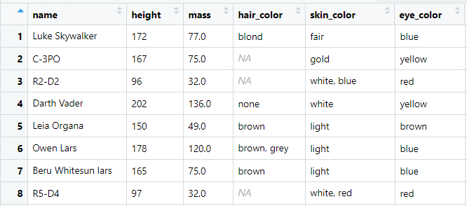
The dataframe contains 87 rows and 14 variables related to different characters from the Star Wars franchise. This dataframe is available as one of the toy dataframes one can use to play with the dplyr library — we’ll use it to understand the behavior of our dplyr functions and play around with some examples.

The first dplyr function that we will learn is filter . This function is widely used to filter rows from dataframes using one or multiple conditions.

Filter is a really cool function to subset rows from dataframes — for instance, let’s filter all species that are Droid in the starwarstable:

filter_droids <- starwars %>%
filter(species == 'Droid')

This code outputs the 7 characters out of the Star Wars franchise data:

We could use indexes in base R to achieve exactly the same thing — with one big caveat:

starwars[starwars$species == ‘Droid’,]

The code above would yield some NA’s — you would have to add an extra condition to only subset the Droid Species. This is one of the main advantages (removing NA’s automatically) of using the filter function — other than being accessible via %>% .

Another cool feature of the filter function is that we can add more conditions neatly — for instance, let’s just select Droidswith gold “skin” color:

filter_droids_gold <- starwars %>%
filter(species == ‘Droid’, skin_color == ‘gold’)

This only outputs a single droid — C3PO!

Just by adding new arguments to the function we are providing more conditions. This feature from the filter function makes your code, arguably, better to read and to debug — particularly when you have complex filters.

arrange sorts our table according to specific columns. For instance, if we want to sort our starwars dataframe by height, we just have to type:

sorted_height <- starwars %>%
arrange(height)

The table output:

We have our table sorted by the height column, starting from the shortest character to the tallest one.

How could we reverse the height order? Super simple, we just have to add a - before the column:

reverse_sorted_height <- starwars %>%
arrange(-height)

In this case, we obtain the data sorted descendingly — in the output, we can see that Yarael Poof is the tallest one, which makes sense!

In base R, you can emulate table sorting using order and indexing:

starwars[order(starwars$height),]

One caveat of using base R is that our code gets messy very fast when we want to sort by multiple columns.

In dplyr , that’s simple and you’ve probably guessed how— we just add a new argument to the arrange function!

sorted_hair_height <- starwars %>%
arrange(hair_color, height)

In this case, we output our characters in the following order:

• first, we sort the character by hair_color, alphabetically.
• By each hair_color, the sort is applied by height.

arrangeis pretty cool because we can sort our table conveniently with a simple function. Additionally, the fact that we can add more columns to the sort order by simply adding new arguments makes arrange a go-to function when you want to perform sort operations.

mutate is a cool function to add new columns to a table.

For instance, let’s imagine I would like to add a new column to the star wars table with a multiplication of two columns — height and mass. Let’s call that column height_x_mass :

starwars_df <- starwars %>%
mutate(height_x_mass = height*mass)

In the example above, I write the result in a new table starwars_dfbecause the existing columns are preserved in the mutate function. What mutatedoes is just adding a new column to the existing dataframe.

Let’s see the resulting object of the code above — scrolling until the last column of our R previewer:

If you scroll to the end of the R dataframe previewer, you can see our new column created!

This column is the calculation of height times mass . Let’s check an example for the first row that contains data regarding the franchise protagonist — Luke Skywalker .

Luke is 172 cm tall and weighs 77 kilograms:

We are expecting that the height_x_mass of Luke to be 172*77, 13.244. Is this the value we obtain on the last column of the first row? Let’s check again:

It is!

With mutate we can create new columns based on existing information or with completely new values. Also, do you think we can add multiple columns at the same time?

Let’s see!

starwars_df <- starwars %>%
mutate(height_x_mass = height*mass,
franchise = ‘Star Wars’)

Nice! We can add multiple columns at the same time just by adding a new argument to the function — sounds familiar? This is why dplyris so flexible!

Note that, on the example above, we’ve added two new columns:

• A column with the height_x_mass , as we’ ve discussed.
• a new column called franchise that contains the string “Star Wars” for all rows.

When you use R to perform some Data Science, Statistics or Analytics projects, you will probably have to do some type of sampling throughout your pipeline.

With R base, one has to play around with indexes, something that is a bit error-prone.

Luckily, dplyrhas two really cool functions to perform samples:

• sample_n that samples random rows from a data frame based on a number of elements.
• sample_frac that samples random rows from a data frame based on the percentage of the original rows of the data frame.

Let’s see!

starwars_sample_n <- starwars %>%
sample_n(size=5)

Notice that the output of the sample_nfunction gives us 5 rows — the number of the size argument. With sample_frac, instead of retrieving an “integer number of rows”, we retrieve a percentage of the original rows — for instance, if we want to obtain 1% of the rows, we can just provide:

starwars_sample_frac <- starwars %>%
sample_frac(0.01)

Why do we only see one row in the output?

The originalstarwars dataframe contains 87 rows. How much is 1% of 87? 0.87. This number is rounded up and we end up retrieving only 1 row from the table.

If we give 0.02 to the sample_n function, can you guess how many rows we would retrieve?

starwars_sample_frac <- starwars %>%
sample_frac(0.02)

0.02 * 87 is equal to 1.74 so we sample 2 rows from the table!

sample_n and sample_frac are pretty cool because you can jump easily between sampling methods only by changing a small portion of your code.

summarise is a really handy wrapper to write summary functions. For instance, imagine we would want to obtain the mean of the height variable — using base R we could:

mean(starwars$height, na.rm=TRUE)

This would be technically correct — we use na.rm to remove the NA’s from the column values and then we apply the mean to the vector. In summarise , we can do the following:

starwars %>%
summarise(height_mean = mean(height, na.rm = TRUE))

This outputs ~174 as well, the mean of the height column. There are two cool features of using summarise vs. base R:

• The first feature is that we can jump through different functions inside summarise:

starwars %>%
summarise(height_max = max(height, na.rm = TRUE))

I changed the function to calculate the max of the column instead of the mean . You can check here some of the built-in functions supported by summarise.

• The second cool feature and, probably, the most useful, is the fact that you can encapsulate summary functions with group_by to produce values per groups. For instance, if I want to check the mean by Species , I just have to:

mean_height_by_species <- starwars %>%
group_by(species) %>%
summarise(height_mean = mean(height, na.rm = TRUE))

Cool! I can perform a group_by immediately before my summarise and this outputs the mean of the height by each species of character. Let’s see the output dataframe:

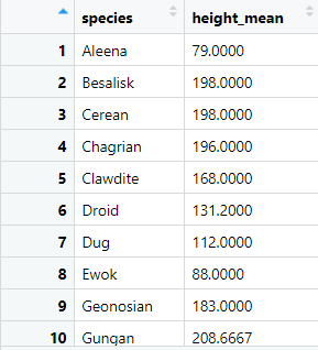
For each species we have a height_mean . This gives us an overview of the average height of all the characters of each specific species in the dataframe. For instance, from the preview, Ewoks and Aleenas are the species with shortest average height and that makes sense!

Combining summarise and other dplyr instructions is pretty common when you are building data pipelines.

If you are familiar with SQL, in the example above we’ve mimicked the behavior of the GROUP BY clause with 3 lines of code. This is an example of something that is much easier to using dplyr than base R.

Speaking of SQL , dplyr has some interesting functions to perform dataframe joins.

Imagine we have an aux dataframe with the fictional origin of each species with the following data:

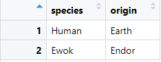
The species_origin dataframe contains information about a fictional origin of a species in the Star Wars franchise. Can we combine this dataframe with the starwars dataframe using joins?

We can do it using the join functions available in dplyr ! Let’s start with an inner_join :

starwars_inner <- starwars %>%
inner_join(species_origin, on=’Species’)

The inner_join functions performs a join between the table before the %>% and the first argument of the function. In this case, we are joining the starwars and the species_origin dataframes by the Species column.

This join outputs 36 observations and an extra column that was added:

Notice that we’ve added the origin column to our starwars dataframe. Naturally, the inner join only returns two species: Human and Ewok . As we are performing an inner_join , we only returns rows where the key is in both dataframes.

If we perform a left_join , the domain of our dataframe changes:

starwars_left <- starwars %>%
left_join(species_origin, on=’Species’)

In this case, the returning dataframe contains 87 rows with the additional column. What happens to the origin column when we can’t find that information in the species_origin ? Let’s see:

It is assigned to a NA value! Although we bring all the rows from the table on the left (the dataframe before the %>% ), the species that don’t have a match on the species_origin dataframe have a NA value on the origin.

Similar to inner_join and left_join , we also have a right_joinavailable in dplyr :

starwars_right <- starwars %>%
right_join(species_origin, on=’Species’)

In the right join, the main table is the one stated in the first argument of the function — species_origin .

For SQL users, these dplyr functions will make their transition to R a bit easier as they can perform joins with a logic that is similar to most SQL implementations.

In this post, we will check some important functions available in one the coolest R data wrangling libraries — dplyr

Dplyr is a really handy library you can use in R. Dplyr is a data manipulation package that is part of the tidyverse universe, a collection of libraries that has the goal of making R faster, simpler and easier.

Other than the cool functions you can access by installing the package, Dplyr leverages the pipe (%>%) structure, a better way to encapsulate functions. Arguably, pipes make your R code easier to debug and understand — sometimes, at the expense of some speed.

The library has dozens of functions available to perform data manipulation and wrangling — in this post, we are going to explore the following ones:

• filter — filters rows;
• arrange — sorts a dataframe;
• mutate — creates new columns;
• sample_n —samples n rows from a dataframe;
• sample_frac — samples a percentage of rows from a dataframe;
• summarize — performs aggregate functions;
• group_by — groups data by a specific key;
• inner, left and right_join —combines multiple dataframes by key;

Throughout this post and for some of the functions, we’ll also compare how to achieve the same goal using R base code — in most cases, this will help us understand the benefits of using dplyr in some R operations.

We’ll perform our examples using the starwars dataframe, a built-in data set that you can use immediately after running library(dplyr) .

Before we start, don’t forget to install and load the dplyr library in R:

# Installing the dplyr Package
install.packages('dplyr')# Loading the library
library(dplyr)

Previewing our starwars dataframe:

The dataframe contains 87 rows and 14 variables related to different characters from the Star Wars franchise. This dataframe is available as one of the toy dataframes one can use to play with the dplyr library — we’ll use it to understand the behavior of our dplyr functions and play around with some examples.

The first dplyr function that we will learn is filter . This function is widely used to filter rows from dataframes using one or multiple conditions.

Filter is a really cool function to subset rows from dataframes — for instance, let’s filter all species that are Droid in the starwarstable:

filter_droids <- starwars %>%
filter(species == 'Droid')

This code outputs the 7 characters out of the Star Wars franchise data:

We could use indexes in base R to achieve exactly the same thing — with one big caveat:

starwars[starwars$species == ‘Droid’,]

The code above would yield some NA’s — you would have to add an extra condition to only subset the Droid Species. This is one of the main advantages (removing NA’s automatically) of using the filter function — other than being accessible via %>% .

Another cool feature of the filter function is that we can add more conditions neatly — for instance, let’s just select Droidswith gold “skin” color:

filter_droids_gold <- starwars %>%
filter(species == ‘Droid’, skin_color == ‘gold’)

This only outputs a single droid — C3PO!

Just by adding new arguments to the function we are providing more conditions. This feature from the filter function makes your code, arguably, better to read and to debug — particularly when you have complex filters.

arrange sorts our table according to specific columns. For instance, if we want to sort our starwars dataframe by height, we just have to type:

sorted_height <- starwars %>%
arrange(height)

The table output:

We have our table sorted by the height column, starting from the shortest character to the tallest one.

How could we reverse the height order? Super simple, we just have to add a - before the column:

reverse_sorted_height <- starwars %>%
arrange(-height)

In this case, we obtain the data sorted descendingly — in the output, we can see that Yarael Poof is the tallest one, which makes sense!

In base R, you can emulate table sorting using order and indexing:

starwars[order(starwars$height),]

One caveat of using base R is that our code gets messy very fast when we want to sort by multiple columns.

In dplyr , that’s simple and you’ve probably guessed how— we just add a new argument to the arrange function!

sorted_hair_height <- starwars %>%
arrange(hair_color, height)

In this case, we output our characters in the following order:

• first, we sort the character by hair_color, alphabetically.
• By each hair_color, the sort is applied by height.

arrangeis pretty cool because we can sort our table conveniently with a simple function. Additionally, the fact that we can add more columns to the sort order by simply adding new arguments makes arrange a go-to function when you want to perform sort operations.

mutate is a cool function to add new columns to a table.

For instance, let’s imagine I would like to add a new column to the star wars table with a multiplication of two columns — height and mass. Let’s call that column height_x_mass :

starwars_df <- starwars %>%
mutate(height_x_mass = height*mass)

In the example above, I write the result in a new table starwars_dfbecause the existing columns are preserved in the mutate function. What mutatedoes is just adding a new column to the existing dataframe.

Let’s see the resulting object of the code above — scrolling until the last column of our R previewer:

If you scroll to the end of the R dataframe previewer, you can see our new column created!

This column is the calculation of height times mass . Let’s check an example for the first row that contains data regarding the franchise protagonist — Luke Skywalker .

Luke is 172 cm tall and weighs 77 kilograms:

We are expecting that the height_x_mass of Luke to be 172*77, 13.244. Is this the value we obtain on the last column of the first row? Let’s check again:

It is!

With mutate we can create new columns based on existing information or with completely new values. Also, do you think we can add multiple columns at the same time?

Let’s see!

starwars_df <- starwars %>%
mutate(height_x_mass = height*mass,
franchise = ‘Star Wars’)

Nice! We can add multiple columns at the same time just by adding a new argument to the function — sounds familiar? This is why dplyris so flexible!

Note that, on the example above, we’ve added two new columns:

• A column with the height_x_mass , as we’ ve discussed.
• a new column called franchise that contains the string “Star Wars” for all rows.

When you use R to perform some Data Science, Statistics or Analytics projects, you will probably have to do some type of sampling throughout your pipeline.

With R base, one has to play around with indexes, something that is a bit error-prone.

Luckily, dplyrhas two really cool functions to perform samples:

• sample_n that samples random rows from a data frame based on a number of elements.
• sample_frac that samples random rows from a data frame based on the percentage of the original rows of the data frame.

Let’s see!

starwars_sample_n <- starwars %>%
sample_n(size=5)

Notice that the output of the sample_nfunction gives us 5 rows — the number of the size argument. With sample_frac, instead of retrieving an “integer number of rows”, we retrieve a percentage of the original rows — for instance, if we want to obtain 1% of the rows, we can just provide:

starwars_sample_frac <- starwars %>%
sample_frac(0.01)

Why do we only see one row in the output?

The originalstarwars dataframe contains 87 rows. How much is 1% of 87? 0.87. This number is rounded up and we end up retrieving only 1 row from the table.

If we give 0.02 to the sample_n function, can you guess how many rows we would retrieve?

starwars_sample_frac <- starwars %>%
sample_frac(0.02)

0.02 * 87 is equal to 1.74 so we sample 2 rows from the table!

sample_n and sample_frac are pretty cool because you can jump easily between sampling methods only by changing a small portion of your code.

summarise is a really handy wrapper to write summary functions. For instance, imagine we would want to obtain the mean of the height variable — using base R we could:

mean(starwars$height, na.rm=TRUE)

This would be technically correct — we use na.rm to remove the NA’s from the column values and then we apply the mean to the vector. In summarise , we can do the following:

starwars %>%
summarise(height_mean = mean(height, na.rm = TRUE))

This outputs ~174 as well, the mean of the height column. There are two cool features of using summarise vs. base R:

• The first feature is that we can jump through different functions inside summarise:

starwars %>%
summarise(height_max = max(height, na.rm = TRUE))

I changed the function to calculate the max of the column instead of the mean . You can check here some of the built-in functions supported by summarise.

• The second cool feature and, probably, the most useful, is the fact that you can encapsulate summary functions with group_by to produce values per groups. For instance, if I want to check the mean by Species , I just have to:

mean_height_by_species <- starwars %>%
group_by(species) %>%
summarise(height_mean = mean(height, na.rm = TRUE))

Cool! I can perform a group_by immediately before my summarise and this outputs the mean of the height by each species of character. Let’s see the output dataframe:

For each species we have a height_mean . This gives us an overview of the average height of all the characters of each specific species in the dataframe. For instance, from the preview, Ewoks and Aleenas are the species with shortest average height and that makes sense!

Combining summarise and other dplyr instructions is pretty common when you are building data pipelines.

If you are familiar with SQL, in the example above we’ve mimicked the behavior of the GROUP BY clause with 3 lines of code. This is an example of something that is much easier to using dplyr than base R.

Speaking of SQL , dplyr has some interesting functions to perform dataframe joins.

Imagine we have an aux dataframe with the fictional origin of each species with the following data:

The species_origin dataframe contains information about a fictional origin of a species in the Star Wars franchise. Can we combine this dataframe with the starwars dataframe using joins?

We can do it using the join functions available in dplyr ! Let’s start with an inner_join :

starwars_inner <- starwars %>%
inner_join(species_origin, on=’Species’)

The inner_join functions performs a join between the table before the %>% and the first argument of the function. In this case, we are joining the starwars and the species_origin dataframes by the Species column.

This join outputs 36 observations and an extra column that was added:

Notice that we’ve added the origin column to our starwars dataframe. Naturally, the inner join only returns two species: Human and Ewok . As we are performing an inner_join , we only returns rows where the key is in both dataframes.

If we perform a left_join , the domain of our dataframe changes:

starwars_left <- starwars %>%
left_join(species_origin, on=’Species’)

In this case, the returning dataframe contains 87 rows with the additional column. What happens to the origin column when we can’t find that information in the species_origin ? Let’s see:

It is assigned to a NA value! Although we bring all the rows from the table on the left (the dataframe before the %>% ), the species that don’t have a match on the species_origin dataframe have a NA value on the origin.

Similar to inner_join and left_join , we also have a right_joinavailable in dplyr :

starwars_right <- starwars %>%
right_join(species_origin, on=’Species’)

In the right join, the main table is the one stated in the first argument of the function — species_origin .

For SQL users, these dplyr functions will make their transition to R a bit easier as they can perform joins with a logic that is similar to most SQL implementations.