
A Comprehensive Guide To Common Machine-Learning Preprocessing Techniques | by Emmett Boudreau | Jul, 2022
An overview and story of various different preprocessing techniques, as well as where they apply in machine-learning
A very common misconception that new and aspiring Data Scientists often have when entering the domain is that most of Data Science revolves around artificial intelligence, machine-learning, and other popular and obscure buzzwords. While many of these buzzwords are certainly different aspects of Data Science, and we really do program machine-learning models, the majority of the job is typically devoted to other tasks. One aspect of Data Science that is unique in comparison to many other technical fields is that Data Science is a collection of different domains and subjects pulled into one field of work. Furthermore, Data Science can be more varied, some Data Scientists might do all of their work exclusively on data-pipelines, and others might work exclusively on neural networks. Some Data Scientists are even hyper-focused on visualizations, dashboards, and statistical tests — for business, medicine, biology, and other domains.
While it might not be common to only do one thing as a Data Scientist, there is one universal thing that all Data Scientists do;
work with data.
Working with data usually involves several key steps, including data wrangling, cleaning, formatting, exploration, and preprocessing. When it comes to getting started with data, and creating some sort of analysis of data, it is typical to wrangle, clean, format, and explore that data. However, preprocessing is a bit more of an interesting case, as preprocessing methods take our data techniques into an entirely new direction. Whereas with the other operations, cleaning, formatting, exploring, we are trying to interpret the data as humans, in the case of preprocessing we have interpreted the data as humans and are now trying to make the data more interpretable for a statistical algorithm. That being said, the amount of preprocessing, along with its effectiveness, can have a serious impact on the performance of a machine-learning model. Given this importance, today we will go through the most popular preprocessing techniques, explain how they work and what they do, and then we will be writing some of them ourselves in order to better demonstrate how they work.
Types Of Features — A brief review
In order to really understand different preprocessing techniques, we first need to have an at least moderate understanding of the data we are actually using the techniques on. Within the world of data, there are several feature types which include primarily continuous, label, and categorical features. Continuous features are described as features where each observation holds numerical value. That being said, continuous features are almost always real, imaginary, or complex numbers — and when they are not, they are a representation of a number. Categorical features on the other hand can encompass a broad array of types, including different numbers and strings. Labels can also be of any type, but are typically either a String or a Date .
An example of a continuous feature would be observations of daily ice-cream sales from an ice-cream truck. If we were to also log the most popular daily flavor of icecream, this would be a categorical feature. Finally, a date would be considered a label for this data. Understanding these different types of features is going to be incredibly important when it comes to using preprocessing methods. This also is going to be incredibly important when it comes to understanding the data, as there are situations where the feature type is not as obvious at first glance.
Train Test Split
The first preprocessing technique is not necessarily a typical preprocessor. Train test split is a technique that is used to test model’s performance by creating two separate samples. The first sample is a training set, which is used to tell the model how your feature relates to your target, or the thing you are predicting. The test set evaluates how well the model has correlated the feature and the target.
Train test split is relatively straight-forward. Python programmers will likely find train_test_split from sklearn.model_selection a useful method for doing this in Python. As far as programming one yourself goes, the process is relatively straightforward. The input we are looking for is a DataFrame, and the output we are looking for is two DataFrames split at a certain percentage.
using DataFrames
using Random
My function is going to accomplish this by grabbing a random sub-sequence and then separating the DataFrame values based on that random sub-sequence.
function tts(df::DataFrame; at = .75)
sample = randsubseq(1:size(df,1), at)
trainingset = df[sample, :]
notsample = [i for i in 1:size(df,1) if   isempty(searchsorted(sample, i))]
testset = df[notsample, :]
return(trainingset,testset)
end
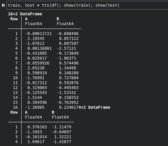
This can easily be achieved using a simple comprehension. Let us now try this function out and see our split data:
df = DataFrame(:A => randn(20), :B => randn(20))train, test = tts(df); show(train); show(test)
Scalers
The next preprocessing technique I wanted to discuss is scalers. Scalers are used on continuous features to form the data into an amount that changes the numerical distance in some way. There are all kinds of different examples of scalers, such as a UniformScaler, and Arbitrary Rescaler, but the most popular type of scaler used in machine-learning is definitely the Standard Scaler. This scaler adjusts the numerical distance of a feature using the normal distribution.
In a normal distribution, every value is instead brought as a relation to the mean. This relation is measured in standard deviations from the mean, so in most cases numbers will come out to be some kind of float that is less than 5. The center of the parabola, where most of our data resides, is made 0. Each value with numerical distance is instead scaled by the number of standard deviations that value is from the mean. This distance is also non-absolute, but statistical significance in the distance is — so the value can be -2, or 2, but both -2 and 2 are statistically significant.
The normal distribution is great for scaling features for machine-learning because it decreases numerical distance, and uses the center of the population as a new reference point. I like to think of it almost like we are creating a new zero, and our new zero is the mean of our population. Given that a standard scaler is simply a normal distribution, the formula for creating one is incredibly simple and exactly the same. First, we will need the both the mean and the standard deviation. For each sample inside of x, we are going to subtract the mean and then divide the difference by the standard deviation.
function standardscale(x::Vector{<:Real})
N::Int64 = length(x)
σ::Number = std(x)
μ::Number = mean(x)
Vector{Real}([i = (i-μ) / σ for i in x])
end
The result is something quite similar to what I discussed earlier, with most of these values residing below 2 in this instance. The reason why all of these values reside below two is because the data is spread out very evenly, as it is just counting numbers:
x = [1, 2, 3, 4, 5, 6, 7, 8, 9, 10]
standardscale(x)
10-element Vector{Real}:
-1.9188064472004938
-1.4924050144892729
-1.066003581778052
-0.6396021490668312
-0.21320071635561041
0.21320071635561041
0.6396021490668312
1.066003581778052
1.4924050144892729
1.9188064472004938
Demonstrating the distribution a bit further, if our first number were to be something completely ridiculous compared to the mean of the population, we would see that the value will grow phenomenally. This will also become an outlier, which will skew the rest of our data away from the mean. This happens because the mean grows in distance from zero whenever a larger number is added:
10-element Vector{Real}:
17.290069740400327
-3.0348109528238902
-2.756387929629038
-2.4779649064341855
-2.199541883239333
-1.9211188600444808
-1.6426958368496287
-1.3642728136547764
-1.085849790459924
-0.8074267672650718
Encoders
Next, we will discuss encoders. Encoders are used to get data that a computer cannot quantitative into data that a computer can quantitative. Encoding is typically reserved for categorical features, but you can also encode labels for interpretation by a computer, which can be useful for things like date strings. Probably the most popular form of encoder used in machine-learning is the one-hot encoder. This encoder turns categorical observations into binary features. Consider the following features:
greeting = ["hello", "hello", "hi"]
age = [34, 17, 21]
The categorical of these two features is the greeting feature. What one hot encoding will do is create a new binary feature for each category. In this case, there are two categories, "hello" and "hi" , so a one-hot encoded version of this feature would be the following two features:
hello = [1, 1, 0]
hi = [0, 0, 1]
What we are doing is checking whether or not each value is of that category, and constructing a BitArray out of that information. To build a function for this, it is as straight forward as typical filtering or masking. We simply need to create a set of BitArrays for each value in the feature’s set:
function onehot(df::DataFrame, symb::Symbol)
dfcopy = copy(df)
[dfcopy[!, Symbol(c)] = dfcopy[!,symb] .== c for c in unique(dfcopy[!,symb])]
dfcopy
end
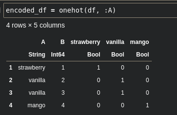
I do this in Julia by broadcasting the == operator to quickly create a Vector .
df = DataFrame(:A => ["strawberry", "vanilla", "vanilla", "mango"],
:B => [1, 2, 3, 4])
encoded_df = onehot(df, :A)show(encoded_df)
Slightly less confusing and easier to understand is the ordinal encoder. This encoder uses the order of the set in order to numerically place each value as a category. Generally, the ordinal encoder is my first choice for categorical applications where there are less categories to worry about. This type of encoding is typically done by creating an element index reference for each category in the feature’s set, and then calling that that reference by key whenever we encounter that value, retrieving the index to replace it with.
function ordinal(df::DataFrame, symb::Symbol)
lookup = Dict(v => i for (i,v) in df[!, symb] |> unique |> enumerate)
map(x->lookup[x], df[!, symb])
endordinal(df, :A)4-element Vector{Int64}:
1
2
2
3
Another encoder that is also really easy to understand is the float encoder. Sometimes also called the label encoder, this encoder turns each Char of a String into a Float . The process for doing so is incredibly simple, and in most cases leaves an encoding that is similar to ordinal encoding, however numbers are not indexes they are instead random jumbles of numbers. Needless to say, this is much more useful to examine labels, as there could be small detectable variations between chars to be read.
function float_encode(df::DataFrame, symb::Symbol)
floatencoded = Vector{Float64}()
for observation in df[!, symb]
s = ""
[s = s * string(float(c)) for c in observation]
s = replace(s, "." => "")
push!(floatencoded, parse(Float64, s))
end
floatencoded
end
For a little more information on encoders in general, as well as the more conventional object-oriented approach to these problems, you may read more about encoders in another article I have written here:
Imputers
Imputers are an easy and automated way to get rid of missing values inside of your data. Imputers typically replace these missing values with the majority class in a categorical problem, or the mean in a continuous problem. What imputers do is take problematic values and turn them into some sort of value with significantly less statistical significance, which is typically the center of the data. We can build a simple mean imputer to replace missing continuous values by simply replacing the value with the mean if it is missing. The only problem is that whenever we try and get the mean of a Vector that has both missing values and numbers, we will get an error because we cannot get the summation of a missing and an integer, for example. As a result, we need to make a bit of an odd function which gives us the mean but skips if the number is missing:
missing_mean(x::Vector) = begin
summation = 0
len = 0
for number in x
if ismissing(number)
continue
end
summation += number
len += 1
end
summation / len
end
Then we will create our imputer by calculating the mean using this function, and then replacing each missing with that mean.
function impute_mean(x::AbstractVector)
μ::Number = missing_mean(x)
[if ismissing(v) μ else v end for v in x]
endx = [5, 10, missing, 20, missing, 82, missing, missing, 40]
impute_mean(x)9-element Vector{Real}:
5
10
31.4
20
31.4
82
31.4
31.4
40
Decomposition
The next major concept in the world of data processing is decomposition. Decomposition allows one to take a feature with multiple dimensions and compress those dimensions down into a single consistent value. This is useful because it can be used to give a model less individual features to worry about while still having those features take statistical effect. This is also incredibly valuable for performance, and is incredibly commonly used in machine-learning. The most popular technique for decomposition is Singular Value Decomposition. There is also another really cool technique called Random Projection. I am not going to go into much detail on these two techniques here, but I have written articles on both of them that may be read for more information:
An overview and story of various different preprocessing techniques, as well as where they apply in machine-learning
A very common misconception that new and aspiring Data Scientists often have when entering the domain is that most of Data Science revolves around artificial intelligence, machine-learning, and other popular and obscure buzzwords. While many of these buzzwords are certainly different aspects of Data Science, and we really do program machine-learning models, the majority of the job is typically devoted to other tasks. One aspect of Data Science that is unique in comparison to many other technical fields is that Data Science is a collection of different domains and subjects pulled into one field of work. Furthermore, Data Science can be more varied, some Data Scientists might do all of their work exclusively on data-pipelines, and others might work exclusively on neural networks. Some Data Scientists are even hyper-focused on visualizations, dashboards, and statistical tests — for business, medicine, biology, and other domains.
While it might not be common to only do one thing as a Data Scientist, there is one universal thing that all Data Scientists do;
work with data.
Working with data usually involves several key steps, including data wrangling, cleaning, formatting, exploration, and preprocessing. When it comes to getting started with data, and creating some sort of analysis of data, it is typical to wrangle, clean, format, and explore that data. However, preprocessing is a bit more of an interesting case, as preprocessing methods take our data techniques into an entirely new direction. Whereas with the other operations, cleaning, formatting, exploring, we are trying to interpret the data as humans, in the case of preprocessing we have interpreted the data as humans and are now trying to make the data more interpretable for a statistical algorithm. That being said, the amount of preprocessing, along with its effectiveness, can have a serious impact on the performance of a machine-learning model. Given this importance, today we will go through the most popular preprocessing techniques, explain how they work and what they do, and then we will be writing some of them ourselves in order to better demonstrate how they work.
Types Of Features — A brief review
In order to really understand different preprocessing techniques, we first need to have an at least moderate understanding of the data we are actually using the techniques on. Within the world of data, there are several feature types which include primarily continuous, label, and categorical features. Continuous features are described as features where each observation holds numerical value. That being said, continuous features are almost always real, imaginary, or complex numbers — and when they are not, they are a representation of a number. Categorical features on the other hand can encompass a broad array of types, including different numbers and strings. Labels can also be of any type, but are typically either a String or a Date .
An example of a continuous feature would be observations of daily ice-cream sales from an ice-cream truck. If we were to also log the most popular daily flavor of icecream, this would be a categorical feature. Finally, a date would be considered a label for this data. Understanding these different types of features is going to be incredibly important when it comes to using preprocessing methods. This also is going to be incredibly important when it comes to understanding the data, as there are situations where the feature type is not as obvious at first glance.
Train Test Split
The first preprocessing technique is not necessarily a typical preprocessor. Train test split is a technique that is used to test model’s performance by creating two separate samples. The first sample is a training set, which is used to tell the model how your feature relates to your target, or the thing you are predicting. The test set evaluates how well the model has correlated the feature and the target.
Train test split is relatively straight-forward. Python programmers will likely find train_test_split from sklearn.model_selection a useful method for doing this in Python. As far as programming one yourself goes, the process is relatively straightforward. The input we are looking for is a DataFrame, and the output we are looking for is two DataFrames split at a certain percentage.
using DataFrames
using Random
My function is going to accomplish this by grabbing a random sub-sequence and then separating the DataFrame values based on that random sub-sequence.
function tts(df::DataFrame; at = .75)
sample = randsubseq(1:size(df,1), at)
trainingset = df[sample, :]
notsample = [i for i in 1:size(df,1) if   isempty(searchsorted(sample, i))]
testset = df[notsample, :]
return(trainingset,testset)
end
This can easily be achieved using a simple comprehension. Let us now try this function out and see our split data:
df = DataFrame(:A => randn(20), :B => randn(20))train, test = tts(df); show(train); show(test)
Scalers
The next preprocessing technique I wanted to discuss is scalers. Scalers are used on continuous features to form the data into an amount that changes the numerical distance in some way. There are all kinds of different examples of scalers, such as a UniformScaler, and Arbitrary Rescaler, but the most popular type of scaler used in machine-learning is definitely the Standard Scaler. This scaler adjusts the numerical distance of a feature using the normal distribution.
In a normal distribution, every value is instead brought as a relation to the mean. This relation is measured in standard deviations from the mean, so in most cases numbers will come out to be some kind of float that is less than 5. The center of the parabola, where most of our data resides, is made 0. Each value with numerical distance is instead scaled by the number of standard deviations that value is from the mean. This distance is also non-absolute, but statistical significance in the distance is — so the value can be -2, or 2, but both -2 and 2 are statistically significant.
The normal distribution is great for scaling features for machine-learning because it decreases numerical distance, and uses the center of the population as a new reference point. I like to think of it almost like we are creating a new zero, and our new zero is the mean of our population. Given that a standard scaler is simply a normal distribution, the formula for creating one is incredibly simple and exactly the same. First, we will need the both the mean and the standard deviation. For each sample inside of x, we are going to subtract the mean and then divide the difference by the standard deviation.
function standardscale(x::Vector{<:Real})
N::Int64 = length(x)
σ::Number = std(x)
μ::Number = mean(x)
Vector{Real}([i = (i-μ) / σ for i in x])
end
The result is something quite similar to what I discussed earlier, with most of these values residing below 2 in this instance. The reason why all of these values reside below two is because the data is spread out very evenly, as it is just counting numbers:
x = [1, 2, 3, 4, 5, 6, 7, 8, 9, 10]
standardscale(x)
10-element Vector{Real}:
-1.9188064472004938
-1.4924050144892729
-1.066003581778052
-0.6396021490668312
-0.21320071635561041
0.21320071635561041
0.6396021490668312
1.066003581778052
1.4924050144892729
1.9188064472004938
Demonstrating the distribution a bit further, if our first number were to be something completely ridiculous compared to the mean of the population, we would see that the value will grow phenomenally. This will also become an outlier, which will skew the rest of our data away from the mean. This happens because the mean grows in distance from zero whenever a larger number is added:
10-element Vector{Real}:
17.290069740400327
-3.0348109528238902
-2.756387929629038
-2.4779649064341855
-2.199541883239333
-1.9211188600444808
-1.6426958368496287
-1.3642728136547764
-1.085849790459924
-0.8074267672650718
Encoders
Next, we will discuss encoders. Encoders are used to get data that a computer cannot quantitative into data that a computer can quantitative. Encoding is typically reserved for categorical features, but you can also encode labels for interpretation by a computer, which can be useful for things like date strings. Probably the most popular form of encoder used in machine-learning is the one-hot encoder. This encoder turns categorical observations into binary features. Consider the following features:
greeting = ["hello", "hello", "hi"]
age = [34, 17, 21]
The categorical of these two features is the greeting feature. What one hot encoding will do is create a new binary feature for each category. In this case, there are two categories, "hello" and "hi" , so a one-hot encoded version of this feature would be the following two features:
hello = [1, 1, 0]
hi = [0, 0, 1]
What we are doing is checking whether or not each value is of that category, and constructing a BitArray out of that information. To build a function for this, it is as straight forward as typical filtering or masking. We simply need to create a set of BitArrays for each value in the feature’s set:
function onehot(df::DataFrame, symb::Symbol)
dfcopy = copy(df)
[dfcopy[!, Symbol(c)] = dfcopy[!,symb] .== c for c in unique(dfcopy[!,symb])]
dfcopy
end
I do this in Julia by broadcasting the == operator to quickly create a Vector .
df = DataFrame(:A => ["strawberry", "vanilla", "vanilla", "mango"],
:B => [1, 2, 3, 4])
encoded_df = onehot(df, :A)show(encoded_df)
Slightly less confusing and easier to understand is the ordinal encoder. This encoder uses the order of the set in order to numerically place each value as a category. Generally, the ordinal encoder is my first choice for categorical applications where there are less categories to worry about. This type of encoding is typically done by creating an element index reference for each category in the feature’s set, and then calling that that reference by key whenever we encounter that value, retrieving the index to replace it with.
function ordinal(df::DataFrame, symb::Symbol)
lookup = Dict(v => i for (i,v) in df[!, symb] |> unique |> enumerate)
map(x->lookup[x], df[!, symb])
endordinal(df, :A)4-element Vector{Int64}:
1
2
2
3
Another encoder that is also really easy to understand is the float encoder. Sometimes also called the label encoder, this encoder turns each Char of a String into a Float . The process for doing so is incredibly simple, and in most cases leaves an encoding that is similar to ordinal encoding, however numbers are not indexes they are instead random jumbles of numbers. Needless to say, this is much more useful to examine labels, as there could be small detectable variations between chars to be read.
function float_encode(df::DataFrame, symb::Symbol)
floatencoded = Vector{Float64}()
for observation in df[!, symb]
s = ""
[s = s * string(float(c)) for c in observation]
s = replace(s, "." => "")
push!(floatencoded, parse(Float64, s))
end
floatencoded
end
For a little more information on encoders in general, as well as the more conventional object-oriented approach to these problems, you may read more about encoders in another article I have written here:
Imputers
Imputers are an easy and automated way to get rid of missing values inside of your data. Imputers typically replace these missing values with the majority class in a categorical problem, or the mean in a continuous problem. What imputers do is take problematic values and turn them into some sort of value with significantly less statistical significance, which is typically the center of the data. We can build a simple mean imputer to replace missing continuous values by simply replacing the value with the mean if it is missing. The only problem is that whenever we try and get the mean of a Vector that has both missing values and numbers, we will get an error because we cannot get the summation of a missing and an integer, for example. As a result, we need to make a bit of an odd function which gives us the mean but skips if the number is missing:
missing_mean(x::Vector) = begin
summation = 0
len = 0
for number in x
if ismissing(number)
continue
end
summation += number
len += 1
end
summation / len
end
Then we will create our imputer by calculating the mean using this function, and then replacing each missing with that mean.
function impute_mean(x::AbstractVector)
μ::Number = missing_mean(x)
[if ismissing(v) μ else v end for v in x]
endx = [5, 10, missing, 20, missing, 82, missing, missing, 40]
impute_mean(x)9-element Vector{Real}:
5
10
31.4
20
31.4
82
31.4
31.4
40
Decomposition
The next major concept in the world of data processing is decomposition. Decomposition allows one to take a feature with multiple dimensions and compress those dimensions down into a single consistent value. This is useful because it can be used to give a model less individual features to worry about while still having those features take statistical effect. This is also incredibly valuable for performance, and is incredibly commonly used in machine-learning. The most popular technique for decomposition is Singular Value Decomposition. There is also another really cool technique called Random Projection. I am not going to go into much detail on these two techniques here, but I have written articles on both of them that may be read for more information:
Denial of responsibility! Techno Blender is an automatic aggregator of the all world’s media. In each content, the hyperlink to the primary source is specified. All trademarks belong to their rightful owners, all materials to their authors. If you are the owner of the content and do not want us to publish your materials, please contact us by email – [email protected]. The content will be deleted within 24 hours.