A Definitive Guide to Using BigQuery Efficiently

By Jessie Hobb On Mar 5, 2024

Make the most out of your BigQuery usage, burn data rather than money to create real value with some practical techniques.

· 📝 Introduction
· 💎 BigQuery basics and understanding costs
∘ Storage
∘ Compute
· 📐 Data modeling
∘ Data types
∘ The shift towards de-normalization
∘ Partitioning
∘ Clustering
∘ Nested repeated columns
∘ Indexing
∘ Physical Bytes Storage Billing
∘ Join optimizations with primary keys and foreign keys
· ⚙️ Data operations
∘ Copy data / tables
∘ Load data
∘ Delete partitions
∘ Get distinct partitions for a table
∘ Do not persist calculated measures
· 📚 Summary
∘ Embrace data modeling best practices
∘ Master data operations for cost-effectiveness
∘ Design for efficiency and avoid unnecessary data persistence

Disclaimer: BigQuery is a product which is constantly being developed, pricing might change at any time and this article is based on my own experience.

Photo by Konstantin Evdokimov on Unsplash

📝 Introduction

In the field of data warehousing, there’s a universal truth: managing data can be costly. Like a dragon guarding its treasure, each byte stored and each query executed demands its share of gold coins. But let me give you a magical spell to appease the dragon: burn data, not money!

In this article, we will unravel the arts of BigQuery sorcery, to reduce costs while increasing efficiency, and beyond. Join as we journey through the depths of cost optimization, where every byte is a precious coin.

💎 BigQuery basics and understanding costs

BigQuery is not just a tool but a package of scalable compute and storage technologies, with fast network, everything managed by Google. At its core, BigQuery is a serverless Data Warehouse for analytical purposes and built-in features like Machine Learning (BigQuery ML). BigQuery separates storage and compute with Google’s Jupiter network in-between to utilize 1 Petabit/sec of total bisection bandwidth. The storage system is using Capacitor, a proprietary columnar storage format by Google for semi-structured data and the file system underneath is Colossus, the distributed file system by Google. The compute engine is based on Dremel and it uses Borg for cluster management, running thousands of Dremel jobs across cluster(s).

BigQuery is not just a tool but a package of scalable compute and storage technologies, with fast network, everything managed by Google

The following illustration shows the basic architecture of how BigQuery is structured:

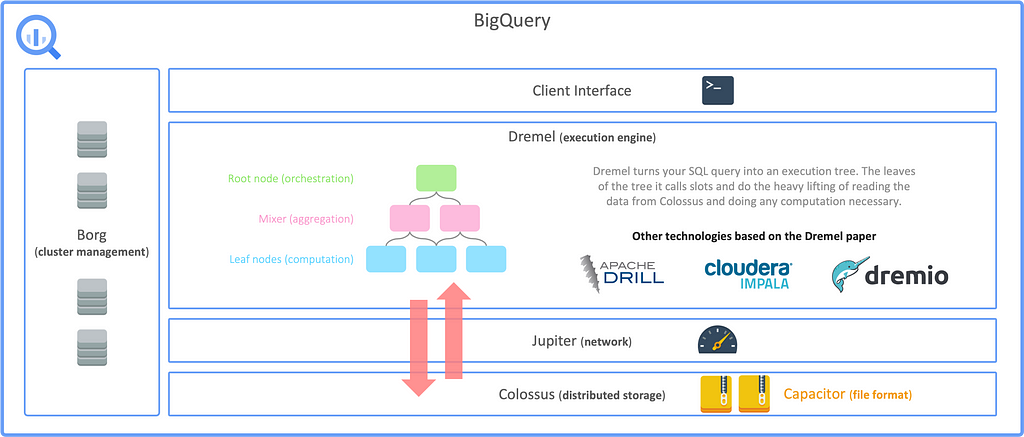
Data can be stored in Colossus, however, it is also possible to create BigQuery tables on top of data stored in Google Cloud Storage. In that case, queries are still processed using the BigQuery compute infrastructure but read data from GCS instead. Such external tables come with some disadvantages but in some cases it can be more cost efficient to have the data stored in GCS. Also, sometimes it is not about Big Data but simply reading data from existing CSV files that are somehow ingested to GCS. For simplicity it can also be benficial to use these kind of tables.

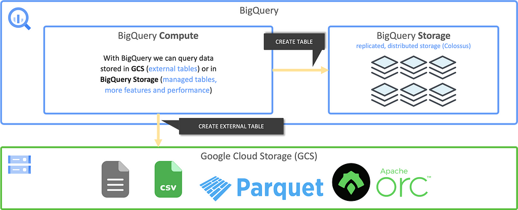
To utilize the full potential of BigQuery, the regular case is to store data in the BigQuery storage.

The main drivers for costs are storage and compute, Google is not charging you for other parts, like the network transfer in between storage and compute.

Storage

Storage costs you $0.02 per GB — $0.04 per GB for active and $0.01 per GB — $0.02 per GB for inactive data (which means not modified in the last 90 days). If you have a table or partition that is not modified for 90 consecutive days, it is considered long term storage, and the price of storage automatically drops by 50%. Discount is applied on a per-table, per-partition basis. Modification resets the 90-day counter.

Compute

BigQuery charges for data scanned and not the runtime of the query, also transfer from storage to compute cluster is not charged. Compute costs depend on the location, the costs for europe-west3 are $8.13 per TB for example.

This means:

We want to minimize the data to be scanned for each query!

Left: Jp Valery on Unsplash, right: Gabriel Jimenez on Unsplash

When executing a query, BigQuery is estimating the data to be processed. After entering your query in the BigQuery Studio query editor, you can see the estimate on the top right.

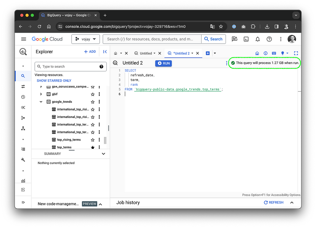
If it says 1.27 GB like in the screenshot above and the query is processed in the location europe-west3, the costs can be calculated like this:

1.27 GB / 1024 = 0.0010 TB * $8.13 = $0.0084 total costs

The estimate is mostly a pessimistic calculation, often the optimizer is able to use cached results, materialized views or other techniques, so that the actual bytes billed are lower than the estimate. It is still a good practice to check this estimate in order to get a rough feeling of the impact of your work.

It is also possible to set a maximum for the bytes billed for your query. If your query exceeds the limit it will fail and create no costs at all. The setting can be changed by navigating to More -> Query settings -> Advanced options -> Maximum bytes billed.

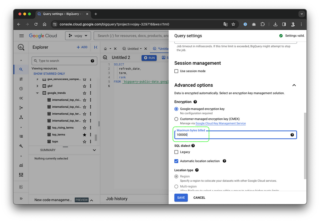
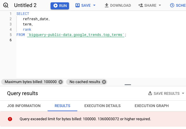
BigQuery exceeded limit for bytes billed

Unfortunately up until now, it is not possible to set a default value per query. It is only possible to limit the bytes billed for each day per user per project or for all bytes billed combined per day for a project.

When you start using BigQuery for the first projects, you will most likely stick with the on-demand compute pricing model. With on-demand pricing, you will generally have access to up to 2000 concurrent slots, shared among all queries in a single project, which is more than enough in most cases. A slot is like a virtual CPU working on a unit of work of your query DAG.

When reaching a certain spending per month, it is worth looking into the capacity pricing model, which gives you more predictable costs.

📐 Data modeling

Data types

To reduce the costs for storage but also compute, it is very important to always use the smallest datatype possible for your columns. You can easily estimate the costs for a certain amount of rows following this overview:

Type       | Size
-----------|---------------------------------------------------------------
ARRAY      | Sum of the size of its elements 
BIGNUMERIC | 32 logical bytes
BOOL       | 1 logical byte
BYTES      | 2 logical bytes + logical bytes in the value
DATE       | 8 logical bytes
DATETIME   | 8 logical bytes
FLOAT64    | 8 logical bytes
GEOGRAPHY  | 16 logical bytes + 24 logical bytes * vertices in the geo type
INT64      | 8 logical bytes
INTERVAL   | 16 logical bytes
JSON       | Logical bytes in UTF-8 encoding of the JSON string
NUMERIC    | 16 logical bytes
STRING     | 2 logical bytes + the UTF-8 encoded string size
STRUCT     | 0 logical bytes + the size of the contained fields
TIME       | 8 logical bytes
TIMESTAMP  | 8 logical bytes

NULL is calculated as 0 logical bytes

Example:

CREATE TABLE gold.some_table (
  user_id INT64,
  other_id INT64,
  some_String STRING, -- max 10 chars
  country_code STRING(2),
  user_name STRING,   -- max 20 chars
  day DATE
);

With this definition and the table of datatypes, it is possible to estimate the logical size of 100,000,000 rows:

100.000.000 rows * (
  8 bytes (INT64) +
  8 bytes (INT64) +
  2 bytes + 10 bytes (STRING) +
  2 bytes + 2 bytes (STRING(2)) +
  2 bytes + 20 bytes (STRING) +
  8 bytes (DATE)
) = 6200000000 bytes / 1024 / 1024 / 1024
  = 5.78 GB

Assuming we are running a SELECT * on this table, it would cost us 5.78 GB / 1024 = 0.0056 TB * $8.13 = $0.05 in europe-west3.

It is a good idea to make these calculations before designing your data model, not only to optimize the datatype usage but also to get an estimate of the costs for the project that you are working on.

The shift towards de-normalization

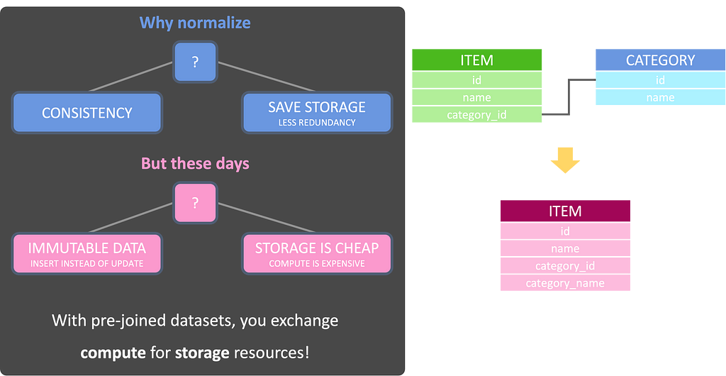
In the realm of database design and management, data normalization and de-normalization are fundamental concepts aimed at optimizing data structures for efficient storage, retrieval, and manipulation. Traditionally, normalization has been hailed as a best practice, emphasizing the reduction of redundancy and the preservation of data integrity. However, in the context of BigQuery and other modern data warehouses, the dynamics shift, and de-normalization often emerges as the preferred approach.

In normalized databases, data is structured into multiple tables, each representing a distinct entity or concept, and linked through relationships such as one-to-one, one-to-many, or many-to-many. This approach adheres to the principles laid out by database normalization forms, such as the First Normal Form (1NF), Second Normal Form (2NF), and Third Normal Form (3NF), among others.

This comes with the advantages of reduction of redundancy, data integrity and consequently, less storage usage.

While data normalization holds merit in traditional relational databases, the paradigm shifts when dealing with modern analytics platforms like BigQuery. BigQuery is designed for handling massive volumes of data and performing complex analytical queries at scale. In this environment, the emphasis shifts from minimizing storage space to optimizing query performance.

In BigQuery, de-normalization emerges as a preferred strategy for several reasons:

Query Performance: BigQuery’s distributed architecture excels at scanning large volumes of data in parallel. De-normalized tables reduce the need for complex joins, resulting in faster query execution times.
Cost Efficiency: By minimizing the computational resources required for query processing, de-normalization can lead to cost savings, as query costs in BigQuery are based on the amount of data processed.
Simplified Data Modeling: De-normalized tables simplify the data modeling process, making it easier to design and maintain schemas for analytical purposes.
Optimized for Analytical Workloads: De-normalized structures are well-suited for analytical workloads, where aggregations, transformations, and complex queries are common.

Also, storage is much cheaper than compute and that means:

With pre-joined datasets, you exchange compute for storage resources!

Partitioning

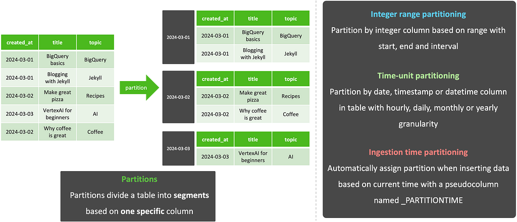
Partitions divide a table into segments based on one specific column. The partition column can use one of 3 approaches:

🗂️ Integer range partitioning: Partition by integer column based on range with start, end and interval

⏰ Time-unit partitioning: Partition by date, timestamp or datetime column in table with hourly, daily, monthly or yearly granularity

⏱️ Ingestion time partitioning: Automatically assign partition when inserting data based on current time with a pseudocolumn named _PARTITIONTIME

It is up to you to define the partition column but it is highly recommend to choose this wisely as it can eliminate a lot of bytes processed / billed.

Example:

CREATE TABLE IF NOT EXISTS silver.some_partitioned_table (
  title STRING,
  topic STRING,
  day DATE
)
PARTITION BY day
OPTIONS (
  partition_expiration_days = 365
);

In the above example you can also see how to set the partition_expiration_days option, which will remove partitions older than X days.

Clustering

Clusters sort the data within each partition based on one ore more columns. When using cluster columns in your query filter, this technique will speed up the execution since BigQuery can determine which blocks to scan. This is especially recommended to use with high cardinality columns such as the title column in the following example.

You can define up to four cluster columns.

Example:

CREATE TABLE IF NOT EXISTS silver.some_partitioned_table (
  title STRING,
  topic STRING,
  day DATE
)
PARTITION BY day
CLUSTER BY topic
OPTIONS (
  partition_expiration_days = 365
);

Nested repeated columns

With data de-normalization often also duplication of information is introduced. This data redundancy adds additional storage and bytes to be processed in our queries. However, there is a way to have a de-normalized table design without redundancy using nested repeated columns.

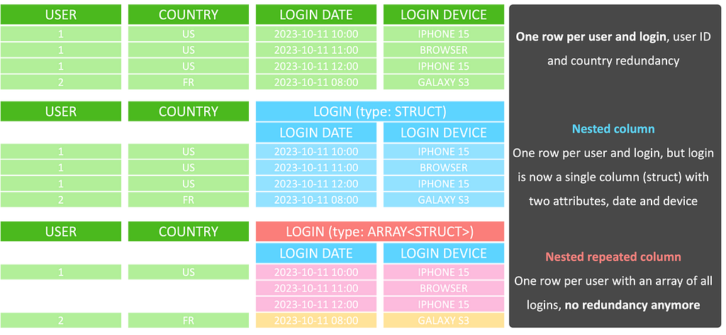
A nested column uses the type struct and combines certain attributes to one object. A nested repeated column is an array of structs stored for a single row in the table. For example: if you have a table storing one row per login of a user, together with the user ID and the registration country of that user, you would have redundancy in form of the ID and country per login for each user.

Instead of storing one row per login, with a nested repeated column you can store one single row per user and in a column of type ARRAY<STRUCT<…>> you store an array of all logins of that user. The struct holds all attributes attached to the login, like the date and device. The following illustration visualizes this example:

Example:

CREATE TABLE silver.logins (
    user_id INT64,
    country STRING(2),
    logins ARRAY<STRUCT<
        login_date DATE,
        login_device STRING
    >>,
    day DATE
)
PARTITION BY day
CLUSTER BY country, user_id
OPTIONS (
    require_partition_filter=true
);

The above example also shows the utilization of the require_partition_filter which will prevent any queries without filtering on the partition column.

This data modelling technique can reduce the stored and processed bytes drastically. However, it is not the silver bullet for all de-normalization or data modeling cases. The major downside is: you can’t set cluster or partition columns on attributes of structs.

That means: in the example above, if a user would filter by login_device a full table scan is necessary and we do not have the option to optimize this with clustering. This can be an issue especially if your table is used as a data source for third party software like Excel or PowerBI. In such cases, you should carefully evaluate if the benefit of removing redundancy with nested repeated columns compensates the lack of optimizations via clustering.

Indexing

By defining a search index on one or multiple columns, BigQuery can use this to speed up queries using the SEARCH function.

A search index can be created with the CREATE SEARCH INDEX statement:

CREATE SEARCH INDEX example_index ON silver.some_table(ALL COLUMNS);

With ALL COLUMNS the index is automatically created for all STRING and JSON columns. It is also possible to be more selective and add a list of column names instead. With the SEARCH function, the index can be utilized to search within all or specific columns:

SELECT * FROM silver.some_table WHERE SEARCH(some_table, 'needle');

A new feature, which is in preview state by the time writing this article, is to also utilize the index for operators such as =, IN, LIKE, and STARTS_WITH. This can be very beneficial for data structures that are directly used by end users via third party tools like PowerBI or Excel to further increase speed and reduce costs for certain filter operations.

More information about this can be found in the official search index documentation.

Physical Bytes Storage Billing

BigQuery offers two billing models for storage: Standard and Physical Bytes Storage Billing. Choosing the right model depends on your data access patterns and compression capabilities.

The standard model is straightforward. You pay a set price per gigabyte of data, with a slight discount for data that hasn’t been modified in 90 days. This is simple to use and doesn’t require managing different storage categories. However, it can be more expensive if your data is highly compressed or if you don’t access it very often.

Physical Bytes Storage Billing takes a different approach. Instead of paying based on how much logical data you store, you pay based on the physical space it occupies on disk, regardless of how often you access it or how well it’s compressed. This model can be significantly cheaper for highly compressed data or data you don’t access frequently. However, it requires you to manage two separate storage classes: one for frequently accessed data and another for long-term storage, which can add complexity.

So, which model should you choose? Here’s a quick guide:

Choose the standard model if:

Your data isn’t highly compressed.
You prefer a simple and easy-to-manage approach.

Choose PBSB if:

Your data is highly compressed.
You’re comfortable managing different storage classes to optimize costs.

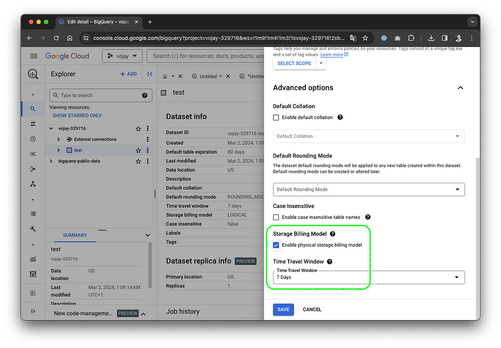
You can change the billing model in the advanced option for your datasets. You can also check the logical vs. physical bytes in the table details view, which makes it easier to decide for a model.

Dataset advanced options for Storage Billing Model

Join optimizations with primary keys and foreign keys

Since July 2023, BigQuery introduced unenforced Primary Key and Foreign Key constraints. Keep in mind that BigQuery is not a classical RDBMS, even though defining a data model with this feature might give you the feeling that it is.

If the keys are not enforced and this is not a relational database as we know it, what is the point? The answer is: the query optimizer may use this information to better optimize queries, namely with the concepts of Inner Join Elimination, Outer Join Elimination and Join Reordering.

Defining constraints is similar to other SQL dialects, just that you have to specify them as NOT ENFORCED:

CREATE TABLE gold.inventory (
 date INT64 REFERENCES dim_date(id) NOT ENFORCED,
 item INT64 REFERENCES item(id) NOT ENFORCED,
 warehouse INT64 REFERENCES warehouse(id) NOT ENFORCED,
 quantity INT64,
 PRIMARY KEY(date, item, warehouse) NOT ENFORCED
);

⚙️ Data operations

Copy data / tables

Copying data from one place to another is a typical part of our daily business as Data Engineers. Let’s assume the task is to copy data from a BigQuery dataset called bronze to another dataset called silver within a Google Cloud Platform project called project_x. The naive approach would be a simple SQL query like:

CREATE OR REPLACE TABLE project_x.silver.login_count AS
SELECT
    user_id,
    platform,
    login_count,
    day
FROM project_x.bronze.login_count;

Even though this allows for transformation, in many cases we simply want to copy data from one place to another. The bytes billed for the query above would essentially be the amount of data we have to read from the source. However, we can also get this for free with the following query:

CREATE TABLE project_x.silver.login_count
COPY project_x.bronze.login_count;

Alternatively, the bq CLI tool can be used to achieve the same result:

bq cp project_x:bronze.login_count project_x:silver.login_count

That way, you can copy data for 0 costs.

Load data

For data ingestion Google Cloud Storage is a pragmatic way to solve the task. No matter if it is a CSV file, ORC / Parquet files from a Hadoop ecosystem or any other source. Data can easily be uploaded and stored for low costs.

It is also possible to create BigQuery tables on top of data stored in GCS. These external tables still utilize the compute infrastructure from BigQuery but do not offer some of the features and performance.

Let’s assume we upload data from a partitioned Hive table using the ORC storage format. Uploading the data can be achieved using distcp or simply by getting the data from HDFS first and then uploading it to GCS using one of the available CLI tools to interact with Cloud Storage.

Assuming we have a partition structure including one partition called month, the files might look like the following:

/some_orc_table/month=2024-01/000000_0.orc
/some_orc_table/month=2024-01/000000_1.orc
/some_orc_table/month=2024-02/000000_0.orc

When we uploaded this data to GCS, an external table definition can be created like this:

CREATE EXTERNAL TABLE IF NOT EXISTS project_x.bronze.some_orc_table
WITH PARTITION COLUMNS
OPTIONS(
  format="ORC",
  hive_partition_uri_prefix="gs://project_x/ingest/some_orc_table",
  uris=["gs://project_x/ingest/some_orc_table/*"]
);

It will derive the schema from the ORC files and even detect the partition column. The naive approach to move this data from GCS to BigQuery storage might now be, to create a table in BigQuery and then follow the pragmatic INSERT INTO … SELECT FROM approach.

However, similar to the previous example, the bytes billed would reflect the amount of data stored in gs://project_x/ingest/some_orc_table. There is another way, which will achieve the same result but again for 0 costs using the LOAD DATA SQL statement.

LOAD DATA OVERWRITE project_x.silver.some_orc_table (
  user_id INT64,
  column_1 STRING,
  column_2 STRING,
  some_value INT64
)
CLUSTER BY column_1, column_2
FROM FILES (
  format="ORC",
  hive_partition_uri_prefix="gs://project_x/ingest/some_orc_table",
  uris=["gs://project_x/ingest/some_orc_table/*"]
)
WITH PARTITION COLUMNS (
  month STRING
);

Using this statement, we directly get a BigQuery table with the data ingested, no need to create an external table first! Also this query comes at 0 costs. The OVERWRITE is optional, since data can also be appended instead of overwriting the table on every run.

As you can see, also the partition columns can be specified. Even though no transformation can be applied, there is one major advantage: we can already define cluster columns. That way, we can create an efficient version of the target table for further downstream processing, for free!

Delete partitions

In certain ETL or ELT scenarios, a typical workflow is to have a table partitioned by day and then replace specific partitions based on new data coming from a staging / ingestion table.

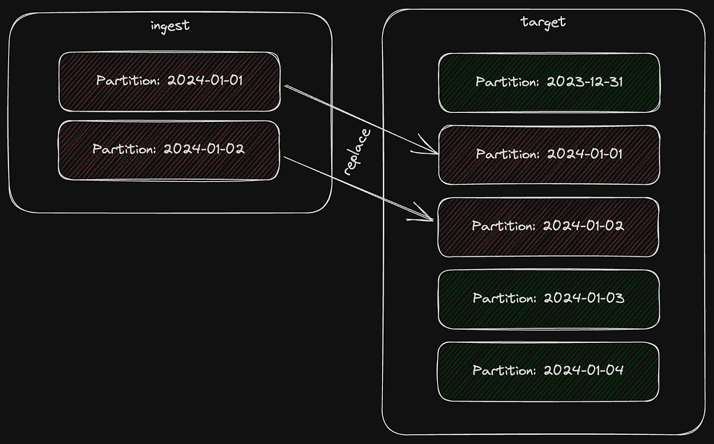
BigQuery offers the MERGE statement but the naive approach is to first delete the affected partitions from the target table and then insert the data.

Deleting partitions in such a scenario can be achieved like this:

DELETE FROM silver.target WHERE day IN (
  SELECT DISTINCT day
  FROM bronze.ingest
);

Even if day is a partition column in both cases, this operation is connected to several costs. However, again there is an alternative solution that comes at 0 costs again:

DROP TABLE silver.target$20240101

With DROP TABLE you can actually also just drop one single partition by appending the suffix $<partition_id>.

Of course the above example is just dropping one partition. However, with the procedual language from BigQuery, we can easily execute the statement in a loop.

FOR x IN (SELECT DISTINCT day FROM bronze.ingest)
DO
  SELECT x; -- replace with DROP TABLE
END FOR;

Or alternatively use Airflow and/or dbt to first select the partitions and then run a certain templated query in a loop.

However, getting the distinct partitions for a partitioned table can be done like the in the examples above, but this will still cause some costs even if we only read a single column. But yet again, there is a way to get this almost for free, which we will explore in the next chapter.

Get distinct partitions for a table

In the examples above, we used the following approach to get the distinct partitions of a partitioned BigQuery table:

SELECT DISTINCT day
FROM bronze.ingest

This is how much the query cost me in an example use-case I worked on:

Bytes billed: 149.14 GB (= $1.18 depending on location)

BigQuery maintains a lot of valuable metadata about tables, columns and partitions. This can be accessed via the INFORMATION_SCHEMA. We can achieve the very same result, by simply using this metadata:

SELECT PARSE_DATE('%Y%m%d', partition_id) AS day
FROM bronze.INFORMATION_SCHEMA.PARTITIONS
WHERE table_name = 'ingest'

And comparing it with the same use-case as I mentioned above, this is how much the query cost:

Bytes billed: 10 MB (= $0.00008 depending on location)

As you can see, 149GB vs 10MB is a huge difference. With this method, you can get the distinct partitions even for huge tables at almost 0 costs.

Do not persist calculated measures

When you start using BigQuery for the first projects, you will most likely stick with the on-demand compute pricing model. With on-demand pricing, you will generally have access to up to 2000 concurrent slots, shared among all queries in a single project. But even with capacity pricing, you will have a minimum of 100 slots.

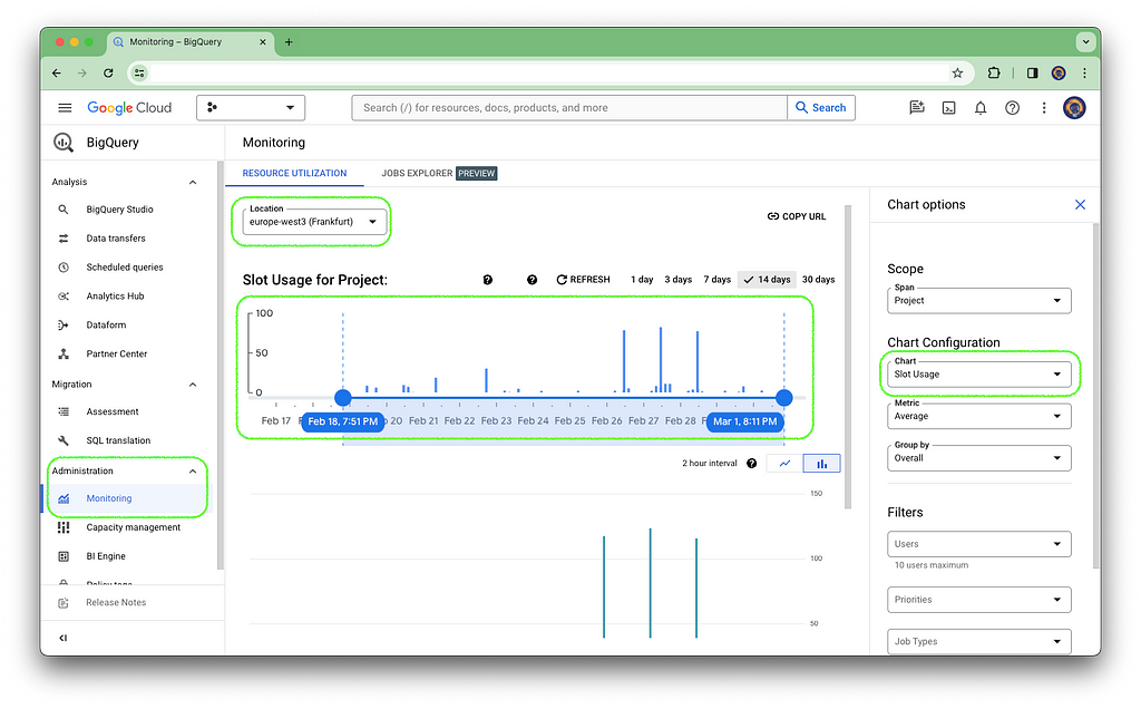
With a lot of the daily ETL / ELT workload, these slots are actually not the limitation of the performance. You can simply check this yourself by navigating to BigQuery -> Administration -> Monitoring, select the correct location and change the Chart to Slot Usage under Chart Configuration. In a lot of cases you will be surprised how little slots you are actually using.

How does that relate to saving costs? Let’s assume you have a classic fact table or some table in general, which delivers certain KPIs. This table is then used for analysis / reporting in Looker, Excel, PowerBI or other tools.

Often these tools automatically generate queries to serve the report or dashboard with the necessary data. These generated queries might not be ideal, when it comes to applying BigQuery best practices. In other words, they might end up scanning more data than necessary which increases the bytes billed.

We can avoid this, by introducing a view layer on top of our fact tables. Serving tools with data from a view rather than the actual table is a very valuable best practice, as it gives you more flexibility when it comes to schema changes but it also gives the possibility to introduce calculated measures within the view without persisting the data.

Of course this might increase the CPU usage when these measures are used but on the other hand, it can drastically reduce the total size of the underlying table.

To illustrate this principle, take the following fact table as a basis:

CREATE TABLE IF NOT EXISTS gold.some_fact_table (
  user_id INT64,
  payment_count INT64,
  value_1 INT64,
  value_2 INT64,
  day DATE
)
PARTITION BY day
CLUSTER BY user_id
OPTIONS (
  partition_expiration_days = 365
);

The basic idea is to introduce a view for stakeholders accessing this data and extend it with calculated measures:

CREATE OR REPLACE VIEW gold.some_fact_view AS
SELECT
  user_id,
  payment_count,
  value_1,
  value_2,
  payment_count > 0 AS is_paying_user,
  value_1 + value_2 AS total_value,
  day
FROM gold.some_fact_table;

In this example we were able to avoid persisting two INT64 values. One of these uses 8 logical bytes. If our fact table has 1,000,000,000 rows this would mean we save:

1000000000 rows * 8 B * 2 columns / 1024 / 1024 / 1024 = 15 GB

This is not a huge amount of data, but it can mean that BigQuery has to scan 15 GB less data in certain situations. In practice, there can be calculated measures that might save you much more data to be scanned.

📚 Summary

Forget hoarding every byte like a dragon guarding its treasure. Instead, learn to burn data through smart management and optimization 🔥. By embracing this fiery approach, you’ll transform BigQuery from a cost center to a powerful engine for data exploration, allowing you to burn data, not money!

Embrace data modeling best practices

Utilize the smallest data types possible to minimize storage and processing costs.
Leverage de-normalization when appropriate to optimize query performance and reduce storage usage.
Implement partitioning and clustering to enable BigQuery to efficiently scan only the relevant data for your queries.
Explore nested repeated columns as a way to eliminate redundancy while maintaining data integrity, but be mindful of limitations regarding clustering.

Master data operations for cost-effectiveness

Employ CREATE TABLE … COPY or bq cp commands to copy data between tables without incurring charges.
Utilize LOAD DATA statements to directly load data from Cloud Storage into BigQuery tables, again at no cost.
Leverage the power of DROP TABLE with partition suffixes to efficiently remove specific partitions.
Utilize INFORMATION_SCHEMA to retrieve table metadata like distinct partition values, significantly reducing costs compared to traditional queries.

Design for efficiency and avoid unnecessary data persistence

Implement a view layer to serve data with calculated measures, preventing the storage of redundant data.
Monitor your BigQuery slot usage to understand if slot limitations are a concern, allowing you to focus on optimizing query structures.

By adopting these strategies, you can unlock the true potential of BigQuery, transforming it into a cost-effective engine for data exploration and analysis. Remember, in the realm of BigQuery, it’s all about burning data, not money!

Feel free to share your experiences in the comments!

A Definitive Guide to Using BigQuery Efficiently was originally published in Towards Data Science on Medium, where people are continuing the conversation by highlighting and responding to this story.

Make the most out of your BigQuery usage, burn data rather than money to create real value with some practical techniques.

Disclaimer: BigQuery is a product which is constantly being developed, pricing might change at any time and this article is based on my own experience.

Photo by Konstantin Evdokimov on Unsplash

📝 Introduction

💎 BigQuery basics and understanding costs

BigQuery is not just a tool but a package of scalable compute and storage technologies, with fast network, everything managed by Google

The following illustration shows the basic architecture of how BigQuery is structured:

To utilize the full potential of BigQuery, the regular case is to store data in the BigQuery storage.

The main drivers for costs are storage and compute, Google is not charging you for other parts, like the network transfer in between storage and compute.

Storage

Compute

This means:

We want to minimize the data to be scanned for each query!

When executing a query, BigQuery is estimating the data to be processed. After entering your query in the BigQuery Studio query editor, you can see the estimate on the top right.

If it says 1.27 GB like in the screenshot above and the query is processed in the location europe-west3, the costs can be calculated like this:

1.27 GB / 1024 = 0.0010 TB * $8.13 = $0.0084 total costs

When reaching a certain spending per month, it is worth looking into the capacity pricing model, which gives you more predictable costs.

📐 Data modeling

Data types

Type       | Size
-----------|---------------------------------------------------------------
ARRAY      | Sum of the size of its elements 
BIGNUMERIC | 32 logical bytes
BOOL       | 1 logical byte
BYTES      | 2 logical bytes + logical bytes in the value
DATE       | 8 logical bytes
DATETIME   | 8 logical bytes
FLOAT64    | 8 logical bytes
GEOGRAPHY  | 16 logical bytes + 24 logical bytes * vertices in the geo type
INT64      | 8 logical bytes
INTERVAL   | 16 logical bytes
JSON       | Logical bytes in UTF-8 encoding of the JSON string
NUMERIC    | 16 logical bytes
STRING     | 2 logical bytes + the UTF-8 encoded string size
STRUCT     | 0 logical bytes + the size of the contained fields
TIME       | 8 logical bytes
TIMESTAMP  | 8 logical bytes

NULL is calculated as 0 logical bytes

Example:

CREATE TABLE gold.some_table (
  user_id INT64,
  other_id INT64,
  some_String STRING, -- max 10 chars
  country_code STRING(2),
  user_name STRING,   -- max 20 chars
  day DATE
);

With this definition and the table of datatypes, it is possible to estimate the logical size of 100,000,000 rows:

100.000.000 rows * (
  8 bytes (INT64) +
  8 bytes (INT64) +
  2 bytes + 10 bytes (STRING) +
  2 bytes + 2 bytes (STRING(2)) +
  2 bytes + 20 bytes (STRING) +
  8 bytes (DATE)
) = 6200000000 bytes / 1024 / 1024 / 1024
  = 5.78 GB

Assuming we are running a SELECT * on this table, it would cost us 5.78 GB / 1024 = 0.0056 TB * $8.13 = $0.05 in europe-west3.

The shift towards de-normalization

This comes with the advantages of reduction of redundancy, data integrity and consequently, less storage usage.

In BigQuery, de-normalization emerges as a preferred strategy for several reasons:

Query Performance: BigQuery’s distributed architecture excels at scanning large volumes of data in parallel. De-normalized tables reduce the need for complex joins, resulting in faster query execution times.
Cost Efficiency: By minimizing the computational resources required for query processing, de-normalization can lead to cost savings, as query costs in BigQuery are based on the amount of data processed.
Simplified Data Modeling: De-normalized tables simplify the data modeling process, making it easier to design and maintain schemas for analytical purposes.
Optimized for Analytical Workloads: De-normalized structures are well-suited for analytical workloads, where aggregations, transformations, and complex queries are common.

Also, storage is much cheaper than compute and that means:

With pre-joined datasets, you exchange compute for storage resources!

Partitioning

Partitions divide a table into segments based on one specific column. The partition column can use one of 3 approaches:

🗂️ Integer range partitioning: Partition by integer column based on range with start, end and interval

⏰ Time-unit partitioning: Partition by date, timestamp or datetime column in table with hourly, daily, monthly or yearly granularity

⏱️ Ingestion time partitioning: Automatically assign partition when inserting data based on current time with a pseudocolumn named _PARTITIONTIME

It is up to you to define the partition column but it is highly recommend to choose this wisely as it can eliminate a lot of bytes processed / billed.

Example:

CREATE TABLE IF NOT EXISTS silver.some_partitioned_table (
  title STRING,
  topic STRING,
  day DATE
)
PARTITION BY day
OPTIONS (
  partition_expiration_days = 365
);

In the above example you can also see how to set the partition_expiration_days option, which will remove partitions older than X days.

Clustering

You can define up to four cluster columns.

Example:

CREATE TABLE IF NOT EXISTS silver.some_partitioned_table (
  title STRING,
  topic STRING,
  day DATE
)
PARTITION BY day
CLUSTER BY topic
OPTIONS (
  partition_expiration_days = 365
);

Nested repeated columns

Example:

CREATE TABLE silver.logins (
    user_id INT64,
    country STRING(2),
    logins ARRAY<STRUCT<
        login_date DATE,
        login_device STRING
    >>,
    day DATE
)
PARTITION BY day
CLUSTER BY country, user_id
OPTIONS (
    require_partition_filter=true
);

The above example also shows the utilization of the require_partition_filter which will prevent any queries without filtering on the partition column.

Indexing

By defining a search index on one or multiple columns, BigQuery can use this to speed up queries using the SEARCH function.

A search index can be created with the CREATE SEARCH INDEX statement:

CREATE SEARCH INDEX example_index ON silver.some_table(ALL COLUMNS);

SELECT * FROM silver.some_table WHERE SEARCH(some_table, 'needle');

More information about this can be found in the official search index documentation.

Physical Bytes Storage Billing

BigQuery offers two billing models for storage: Standard and Physical Bytes Storage Billing. Choosing the right model depends on your data access patterns and compression capabilities.

So, which model should you choose? Here’s a quick guide:

Choose the standard model if:

Your data isn’t highly compressed.
You prefer a simple and easy-to-manage approach.

Choose PBSB if:

Your data is highly compressed.
You’re comfortable managing different storage classes to optimize costs.

You can change the billing model in the advanced option for your datasets. You can also check the logical vs. physical bytes in the table details view, which makes it easier to decide for a model.

Join optimizations with primary keys and foreign keys

Defining constraints is similar to other SQL dialects, just that you have to specify them as NOT ENFORCED:

CREATE TABLE gold.inventory (
 date INT64 REFERENCES dim_date(id) NOT ENFORCED,
 item INT64 REFERENCES item(id) NOT ENFORCED,
 warehouse INT64 REFERENCES warehouse(id) NOT ENFORCED,
 quantity INT64,
 PRIMARY KEY(date, item, warehouse) NOT ENFORCED
);

⚙️ Data operations

Copy data / tables

CREATE OR REPLACE TABLE project_x.silver.login_count AS
SELECT
    user_id,
    platform,
    login_count,
    day
FROM project_x.bronze.login_count;

CREATE TABLE project_x.silver.login_count
COPY project_x.bronze.login_count;

Alternatively, the bq CLI tool can be used to achieve the same result:

bq cp project_x:bronze.login_count project_x:silver.login_count

That way, you can copy data for 0 costs.

Load data

Assuming we have a partition structure including one partition called month, the files might look like the following:

/some_orc_table/month=2024-01/000000_0.orc
/some_orc_table/month=2024-01/000000_1.orc
/some_orc_table/month=2024-02/000000_0.orc

When we uploaded this data to GCS, an external table definition can be created like this:

CREATE EXTERNAL TABLE IF NOT EXISTS project_x.bronze.some_orc_table
WITH PARTITION COLUMNS
OPTIONS(
  format="ORC",
  hive_partition_uri_prefix="gs://project_x/ingest/some_orc_table",
  uris=["gs://project_x/ingest/some_orc_table/*"]
);

LOAD DATA OVERWRITE project_x.silver.some_orc_table (
  user_id INT64,
  column_1 STRING,
  column_2 STRING,
  some_value INT64
)
CLUSTER BY column_1, column_2
FROM FILES (
  format="ORC",
  hive_partition_uri_prefix="gs://project_x/ingest/some_orc_table",
  uris=["gs://project_x/ingest/some_orc_table/*"]
)
WITH PARTITION COLUMNS (
  month STRING
);

Delete partitions

In certain ETL or ELT scenarios, a typical workflow is to have a table partitioned by day and then replace specific partitions based on new data coming from a staging / ingestion table.

BigQuery offers the MERGE statement but the naive approach is to first delete the affected partitions from the target table and then insert the data.

Deleting partitions in such a scenario can be achieved like this:

DELETE FROM silver.target WHERE day IN (
  SELECT DISTINCT day
  FROM bronze.ingest
);

Even if day is a partition column in both cases, this operation is connected to several costs. However, again there is an alternative solution that comes at 0 costs again:

DROP TABLE silver.target$20240101

With DROP TABLE you can actually also just drop one single partition by appending the suffix $<partition_id>.

Of course the above example is just dropping one partition. However, with the procedual language from BigQuery, we can easily execute the statement in a loop.

FOR x IN (SELECT DISTINCT day FROM bronze.ingest)
DO
  SELECT x; -- replace with DROP TABLE
END FOR;

Or alternatively use Airflow and/or dbt to first select the partitions and then run a certain templated query in a loop.

Get distinct partitions for a table

In the examples above, we used the following approach to get the distinct partitions of a partitioned BigQuery table:

SELECT DISTINCT day
FROM bronze.ingest

This is how much the query cost me in an example use-case I worked on:

Bytes billed: 149.14 GB (= $1.18 depending on location)

SELECT PARSE_DATE('%Y%m%d', partition_id) AS day
FROM bronze.INFORMATION_SCHEMA.PARTITIONS
WHERE table_name = 'ingest'

And comparing it with the same use-case as I mentioned above, this is how much the query cost:

Bytes billed: 10 MB (= $0.00008 depending on location)

As you can see, 149GB vs 10MB is a huge difference. With this method, you can get the distinct partitions even for huge tables at almost 0 costs.

Do not persist calculated measures

When you start using BigQuery for the first projects, you will most likely stick with the on-demand compute pricing model. With on-demand pricing, you will generally have access to up to 2000 concurrent slots, shared among all queries in a single project. But even with capacity pricing, you will have a minimum of 100 slots.

Of course this might increase the CPU usage when these measures are used but on the other hand, it can drastically reduce the total size of the underlying table.

To illustrate this principle, take the following fact table as a basis:

CREATE TABLE IF NOT EXISTS gold.some_fact_table (
  user_id INT64,
  payment_count INT64,
  value_1 INT64,
  value_2 INT64,
  day DATE
)
PARTITION BY day
CLUSTER BY user_id
OPTIONS (
  partition_expiration_days = 365
);

The basic idea is to introduce a view for stakeholders accessing this data and extend it with calculated measures:

CREATE OR REPLACE VIEW gold.some_fact_view AS
SELECT
  user_id,
  payment_count,
  value_1,
  value_2,
  payment_count > 0 AS is_paying_user,
  value_1 + value_2 AS total_value,
  day
FROM gold.some_fact_table;

In this example we were able to avoid persisting two INT64 values. One of these uses 8 logical bytes. If our fact table has 1,000,000,000 rows this would mean we save:

1000000000 rows * 8 B * 2 columns / 1024 / 1024 / 1024 = 15 GB

📚 Summary

Embrace data modeling best practices

Utilize the smallest data types possible to minimize storage and processing costs.
Leverage de-normalization when appropriate to optimize query performance and reduce storage usage.
Implement partitioning and clustering to enable BigQuery to efficiently scan only the relevant data for your queries.
Explore nested repeated columns as a way to eliminate redundancy while maintaining data integrity, but be mindful of limitations regarding clustering.

Master data operations for cost-effectiveness

Employ CREATE TABLE … COPY or bq cp commands to copy data between tables without incurring charges.
Utilize LOAD DATA statements to directly load data from Cloud Storage into BigQuery tables, again at no cost.
Leverage the power of DROP TABLE with partition suffixes to efficiently remove specific partitions.
Utilize INFORMATION_SCHEMA to retrieve table metadata like distinct partition values, significantly reducing costs compared to traditional queries.

Design for efficiency and avoid unnecessary data persistence

Implement a view layer to serve data with calculated measures, preventing the storage of redundant data.
Monitor your BigQuery slot usage to understand if slot limitations are a concern, allowing you to focus on optimizing query structures.

By adopting these strategies, you can unlock the true potential of BigQuery, transforming it into a cost-effective engine for data exploration and analysis. Remember, in the realm of BigQuery, it’s all about burning data, not money!

Feel free to share your experiences in the comments!

A Definitive Guide to Using BigQuery Efficiently was originally published in Towards Data Science on Medium, where people are continuing the conversation by highlighting and responding to this story.

Read original article here

Denial of responsibility! Techno Blender is an automatic aggregator of the all world’s media. In each content, the hyperlink to the primary source is specified. All trademarks belong to their rightful owners, all materials to their authors. If you are the owner of the content and do not want us to publish your materials, please contact us by email – [email protected]. The content will be deleted within 24 hours.