
A Gentle Intro to Causality in a Business Setting | by Giovanni Bruner | May, 2022
Understanding correlation won’t help you with decision making and initiatives measurement in a business setting. A solid grasp of causality is what you need.
Whether you are a Data Scientist dealing with Decision Science, Marketing, Customer Science, or effective A/B testing, Causal Reasoning is a top skill you should master in your career. Disentangling cause-effect relationships is typically overlooked in business and is a largely poorly understood practice. Many key decisions are taken on anectodical evidence, many wrong conclusions are driven by spurious correlations. This can go from spamming customers for no reason to disastrous waste of money due to incorrect initiatives.
Truth is that mastering causality when dealing with human behaviour or socio-economic systems, by definition chaotic and multivariate systems, is damn hard. Yet being able to frame problems in a causal fashion greatly helps give some order to the chaos.
Let’s start with a use case
A very common use case will help make things clear:
Your media company has a subscription-based revenue stream. You offer monthly and yearly plans, the usual stuff. Problem is that in the last few months you have been experiencing a significant drop in renewals. Everybody is in a frenzy about it, so your marketing manager rushes to offer your customers a 20% discount for renewal to the entire customer base, without selecting a control group (so no Randomized Control Trial).
After the campaign you look at a random customer and guess what, they renewed after taking the discount. But here comes the problem, how do you know that they renewed as an effect of your campaign? What if your random customer would have renewed their subscription regardless of the discount? You could certainly go and ask, but often this is impossible. What is also impossible is to determine the counterfactual reality of your single random customer, which is observing what would have happened to their plan had you not sent them a discount.
You are facing the Fundamental Problem of Causal Inference, which is that you can only observe one outcome at a time for each person.
We face this problem every time we make an intervention that does not have a deterministic outcome. An intervention is something that we can manipulate to try to get a different causal outcome. For example, deciding to offer a discount is an intervention, since we can also decide the opposite. On the flipside, gender or ethnicity can be causal effects but do not qualify as interventions, since we cannot change somebody’s gender.
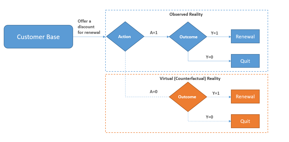
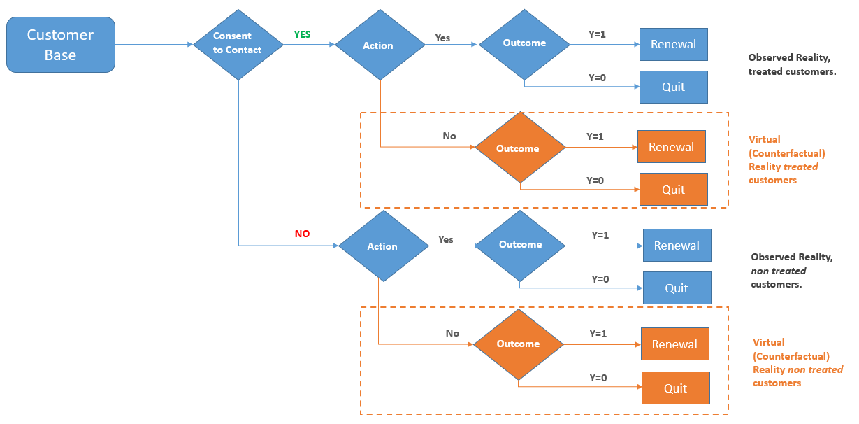
In the figure below we represent this case graphically. In the blue contour what we can observe. You offered a discount to all of our customers, so you can observe two potential outcomes: Y=1 or Y=0. The orange area is the counterfactual world, what would have happened had you not offered the discount. It’s a virtual world you cannot observe directly but on which you can postulate inference.
At this point we can add a bit of notation that will help further down:
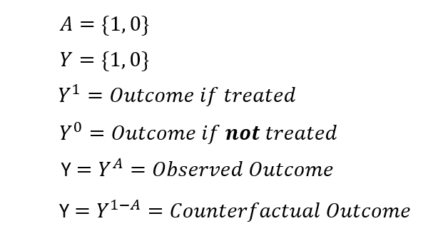
The Action, which from now on we will refer to as the Treatment, can take two possible values, and so does the outcome. We observe an outcome after giving a treatment, the counterfactual is what we would have observed had we not given it. Therefore we have a causal effect only where:

Clearly, if your random customer renewed their membership both in the observed world and in the virtual world, the discount was not necessarily what caused the renewal (the effect).
Estimating the Causal Effect
Estimating the causal effect is the job of scrutinizing the unobservable parallel reality. Or at least making an educating estimate of what happens in there. It can be framed as finding the difference between two expected values:
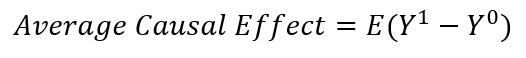
This is the difference between the average outcome for all our customers in the real world and the average outcome in the virtual world, the parallel reality where nobody received a discount for renewing. Only by estimating Y⁰, you do have some chance of correctly measuring the impact of the campaign.
Causality vs Conditioning, the never-ending confusion…
At this point, you might start wondering why we are bothering too much about all of this cause-effect philosophical stuff. After some digging, you find out that not all customers were offered a discount, but only those who had given explicit consent to contact. After all, you might have a control group to measure the campaign’s effectiveness, which makes your finance manager very happy.
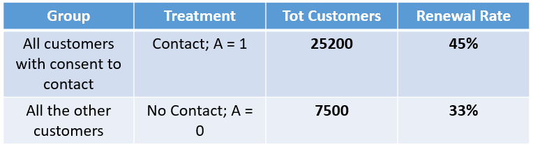
The results in fig 5. are very encouraging, the campaign was a success with 13 pp difference between the two groups. However, your finance manager still finds something fishy about it. As a matter of fact, we need to estimate what a population would have done in a parallel dimension if treated differently than what happened in reality, we are not trying to compare the subpopulation of customers who were treated versus the subpopulation of untreated customers. Put it in math notation:

The average treatment effect is not the same as the difference in outcome between the subpopulation of the treated vs the subpopulation of the non treated.
In essence, as per figure 7. we are interested in inferring what would have happened in the virtual reality for both the subpopulation. We would need to estimate:
- The likely outcome for the customers contacted had they not been contacted. This is the Average Treatment Effect on the Treated (ATT) we defined above.
- The likely outcome for the customer not contacted had they been contacted.
Comparing the two subpopulations is not incorrect in general. It would be fine if we created a Randomized Control Trial from an initial population and a completely random split between the two groups. But in this case, who gets the treatment (the action) depends on providing consent to contact. But who gives the consent to contact for commercial initiatives? Probably people who don’t care about privacy? Or people who intend to be more engaged with your product or website?
Breaking the Ignorability Assumption
After analyzing things further you notice that people who joined the loyalty program are more likely to provide consent to contact and to be involved in a renewal campaign. But guess what, those people are also more likely to spontaneously renew regardless of your campaigns.
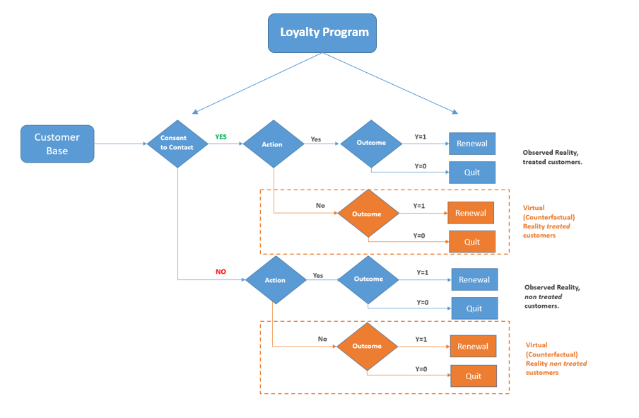
The consent to contact causes your customers to be in the campaign, which in turn causally affects the renewal probability. The loyalty program subscription both affects the consent and the renewal. At this point, we cannot ignore how each customer ended up in the campaign, hence we cannot assume that the treatment assignment was somehow independent of the potential outcome.
As such the loyalty program is a confounder, which is a variable that causes you to be unable of figuring out whether the observed results were due to your marketing prowess or to some backdoor effects of the loyalty program. To clear the confusion, you need to control the confounder by stratifying for this variable.
Let’s expand the campaign outcome by adding a variable X for loyalty program subscriptions. When we add covariates to the groups the situation starts changing.

We can estimate the causal effect of the campaign by comparing the target and the control group along different strata. For those who joined the loyalty program, the campaign was just slightly effective, for the others the campaign had no impact or was slightly detrimental. At this point, we can measure the average treatment effect of the campaign by taking a weighted average of the effects observed at each stratum as shown in fig.9
Identifying and controlling for the right confounders is a step forward toward looking into the virtual reality of counterfactuals. In this example, you don’t know how your campaign’s customers would have behaved without the campaign, but you can make an educated guess by looking at customers similar to them who were not in the campaign. In this case, the loyalty program subscribers who did not provide consent to contact (even if in reality you may want to stratify for many more possible confounders).
The result is that your campaign was less successful than initially anticipated, possibly even generating more costs in giveaway discounts than benefits. Better not tell it to your finance manager.
References:
- I learned most of the ideas and the notation from the wonderful course on Causality by Jason Roy : https://www.coursera.org/learn/crash-course-in-causality
- Another fundamental reference point is The Book of Why: The New Science of Cause and Effect, by Judea Pearl and Dana MacKenzie, Penguin, 2019.
Understanding correlation won’t help you with decision making and initiatives measurement in a business setting. A solid grasp of causality is what you need.
Whether you are a Data Scientist dealing with Decision Science, Marketing, Customer Science, or effective A/B testing, Causal Reasoning is a top skill you should master in your career. Disentangling cause-effect relationships is typically overlooked in business and is a largely poorly understood practice. Many key decisions are taken on anectodical evidence, many wrong conclusions are driven by spurious correlations. This can go from spamming customers for no reason to disastrous waste of money due to incorrect initiatives.
Truth is that mastering causality when dealing with human behaviour or socio-economic systems, by definition chaotic and multivariate systems, is damn hard. Yet being able to frame problems in a causal fashion greatly helps give some order to the chaos.
Let’s start with a use case
A very common use case will help make things clear:
Your media company has a subscription-based revenue stream. You offer monthly and yearly plans, the usual stuff. Problem is that in the last few months you have been experiencing a significant drop in renewals. Everybody is in a frenzy about it, so your marketing manager rushes to offer your customers a 20% discount for renewal to the entire customer base, without selecting a control group (so no Randomized Control Trial).
After the campaign you look at a random customer and guess what, they renewed after taking the discount. But here comes the problem, how do you know that they renewed as an effect of your campaign? What if your random customer would have renewed their subscription regardless of the discount? You could certainly go and ask, but often this is impossible. What is also impossible is to determine the counterfactual reality of your single random customer, which is observing what would have happened to their plan had you not sent them a discount.
You are facing the Fundamental Problem of Causal Inference, which is that you can only observe one outcome at a time for each person.
We face this problem every time we make an intervention that does not have a deterministic outcome. An intervention is something that we can manipulate to try to get a different causal outcome. For example, deciding to offer a discount is an intervention, since we can also decide the opposite. On the flipside, gender or ethnicity can be causal effects but do not qualify as interventions, since we cannot change somebody’s gender.
In the figure below we represent this case graphically. In the blue contour what we can observe. You offered a discount to all of our customers, so you can observe two potential outcomes: Y=1 or Y=0. The orange area is the counterfactual world, what would have happened had you not offered the discount. It’s a virtual world you cannot observe directly but on which you can postulate inference.
At this point we can add a bit of notation that will help further down:
The Action, which from now on we will refer to as the Treatment, can take two possible values, and so does the outcome. We observe an outcome after giving a treatment, the counterfactual is what we would have observed had we not given it. Therefore we have a causal effect only where:
Clearly, if your random customer renewed their membership both in the observed world and in the virtual world, the discount was not necessarily what caused the renewal (the effect).
Estimating the Causal Effect
Estimating the causal effect is the job of scrutinizing the unobservable parallel reality. Or at least making an educating estimate of what happens in there. It can be framed as finding the difference between two expected values:
This is the difference between the average outcome for all our customers in the real world and the average outcome in the virtual world, the parallel reality where nobody received a discount for renewing. Only by estimating Y⁰, you do have some chance of correctly measuring the impact of the campaign.
Causality vs Conditioning, the never-ending confusion…
At this point, you might start wondering why we are bothering too much about all of this cause-effect philosophical stuff. After some digging, you find out that not all customers were offered a discount, but only those who had given explicit consent to contact. After all, you might have a control group to measure the campaign’s effectiveness, which makes your finance manager very happy.
The results in fig 5. are very encouraging, the campaign was a success with 13 pp difference between the two groups. However, your finance manager still finds something fishy about it. As a matter of fact, we need to estimate what a population would have done in a parallel dimension if treated differently than what happened in reality, we are not trying to compare the subpopulation of customers who were treated versus the subpopulation of untreated customers. Put it in math notation:
The average treatment effect is not the same as the difference in outcome between the subpopulation of the treated vs the subpopulation of the non treated.
In essence, as per figure 7. we are interested in inferring what would have happened in the virtual reality for both the subpopulation. We would need to estimate:
- The likely outcome for the customers contacted had they not been contacted. This is the Average Treatment Effect on the Treated (ATT) we defined above.
- The likely outcome for the customer not contacted had they been contacted.
Comparing the two subpopulations is not incorrect in general. It would be fine if we created a Randomized Control Trial from an initial population and a completely random split between the two groups. But in this case, who gets the treatment (the action) depends on providing consent to contact. But who gives the consent to contact for commercial initiatives? Probably people who don’t care about privacy? Or people who intend to be more engaged with your product or website?
Breaking the Ignorability Assumption
After analyzing things further you notice that people who joined the loyalty program are more likely to provide consent to contact and to be involved in a renewal campaign. But guess what, those people are also more likely to spontaneously renew regardless of your campaigns.
The consent to contact causes your customers to be in the campaign, which in turn causally affects the renewal probability. The loyalty program subscription both affects the consent and the renewal. At this point, we cannot ignore how each customer ended up in the campaign, hence we cannot assume that the treatment assignment was somehow independent of the potential outcome.
As such the loyalty program is a confounder, which is a variable that causes you to be unable of figuring out whether the observed results were due to your marketing prowess or to some backdoor effects of the loyalty program. To clear the confusion, you need to control the confounder by stratifying for this variable.
Let’s expand the campaign outcome by adding a variable X for loyalty program subscriptions. When we add covariates to the groups the situation starts changing.
We can estimate the causal effect of the campaign by comparing the target and the control group along different strata. For those who joined the loyalty program, the campaign was just slightly effective, for the others the campaign had no impact or was slightly detrimental. At this point, we can measure the average treatment effect of the campaign by taking a weighted average of the effects observed at each stratum as shown in fig.9
Identifying and controlling for the right confounders is a step forward toward looking into the virtual reality of counterfactuals. In this example, you don’t know how your campaign’s customers would have behaved without the campaign, but you can make an educated guess by looking at customers similar to them who were not in the campaign. In this case, the loyalty program subscribers who did not provide consent to contact (even if in reality you may want to stratify for many more possible confounders).
The result is that your campaign was less successful than initially anticipated, possibly even generating more costs in giveaway discounts than benefits. Better not tell it to your finance manager.
References:
- I learned most of the ideas and the notation from the wonderful course on Causality by Jason Roy : https://www.coursera.org/learn/crash-course-in-causality
- Another fundamental reference point is The Book of Why: The New Science of Cause and Effect, by Judea Pearl and Dana MacKenzie, Penguin, 2019.
Denial of responsibility! Techno Blender is an automatic aggregator of the all world’s media. In each content, the hyperlink to the primary source is specified. All trademarks belong to their rightful owners, all materials to their authors. If you are the owner of the content and do not want us to publish your materials, please contact us by email – [email protected]. The content will be deleted within 24 hours.