
A Guide on Estimating Long-Term Effects in A/B Tests
Addressing the complexity of identifying and measuring long-term effects in online experiments
Imagine you’re an analyst at an online store. You and your team aim to understand how offering free delivery will affect the number of orders on the platform, so you decide to run an A/B test. The test group enjoys free delivery, while the control group sticks to the regular delivery fare. In the initial days of the experiment, you’ll observe more people completing orders after adding items to their carts. But the real impact is long-term — users in the test group are more likely to return for future shopping on your platform because they know you offer free delivery.
In essence, what’s the key takeaway from this example? The impact of free delivery on orders tends to increase gradually. Testing it for only a short period might mean you miss the whole story, and this is a challenge we aim to address in this article.
Understanding Why Long-Term and Short-Term Effects May Differ
Overall, there could be multiple reasons why short-term effects of the experiment differ from long-term effects [1]:
Heterogeneous Treatment Effect
- The impact of the experiment may vary for frequent and occasional users of the product. In the short run, frequent users might disproportionately influence the experiment’s outcome, introducing bias to the average treatment effect.
User Learning
- Novelty Effect — picture this: you introduce a new gamification mechanic to your product. Initially, users are curious, but this effect tends to decrease over time.
- Primacy Effect — think about when Facebook changed its ranking algorithm from chronological to recommendations. Initially, there might be a drop in time spent in the feed as users can’t find what they expect, leading to frustration. However, over time, engagement is likely to recover as users get used to the new algorithm, and discover interesting posts. Users may initially react negatively but eventually adapt, leading to increased engagement.
In this article, our focus will be on addressing two questions:
How to identify and test whether the long-term impact of the experiment differs from the short-term?
How to estimate the long-term effect when running the experiment for a sufficiently long period isn’t possible?
Methods for Identifying Trends in Long-Term Effects
Visualization
The initial step is to observe how the difference between the test and control groups changes over time. If you notice a pattern like this, you will have to dive into the details to grasp the long-term effect.

It might be also tempting to plot the experiment’s effect based not only on the experiment day but also on the number of days from the first exposure.
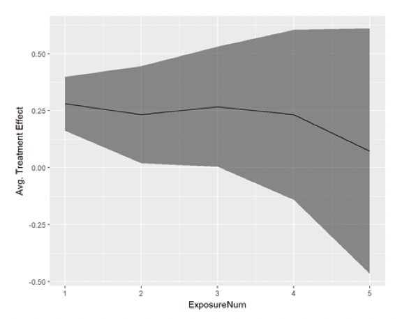
However, there are several pitfalls when you look at the number of days from the first exposure:
- Engaged Users Bias: The right side of the chart might show more engaged users. The observed pattern might not be due to user learning but because of diverse treatment effects. The impact on highly engaged users could be different from the effect on occasional users.
- Selective Sampling Issue: We could decide to focus solely on highly engaged users and observe how their effect evolves over time. However, this subset may not accurately represent the entire user base.
- Decreasing User Numbers: There may be only a few users who have a substantial number of days since the first exposure (the right part of the graph). This widens the confidence intervals, making it tricky to draw dependable conclusions.
The visual method for identifying long-term effects in an experiment is quite straightforward, and it’s always a good starting point to observe the difference in effects over time. However, this approach lacks rigor; you might also consider formally testing the presence of long-term effects. We’ll explore that in the next part.
Ladder Experiment Assignment [2]
The concept behind this approach is as follows: before initiating the experiment, we categorize users into k cohorts and incrementally introduce them to the experiment. For instance, if we divide users into 4 cohorts, k_1 is the control group, k_2 receives the treatment from week 1, k_3 from week 2, and k_4 from week 3.

The user-learning rate can be estimated by comparing the treatment effects from various time periods.
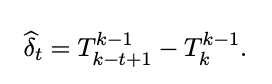
For instance, if you aim to estimate user learning in week 4, you would compare values T4_5 and T4_2.
The challenges with this approach are quite evident. Firstly, it introduces extra operational complexities to the experiment design. Secondly, a substantial number of users are needed to effectively divide them into different cohorts and attain reasonable statistical significance levels. Thirdly, one should anticipate having different long-term effects beforehand, and prepare to run an experiment in this complicated setting.
Difference-in-Difference [2]
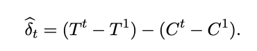
This approach is a simplified version of the previous one. We split the experiment into two (or more generally, into k) time periods and compare the treatment effect in the first period with the treatment effect in the k-th period.
In this approach, a vital question is how to estimate the variance of the estimate to make conclusions about statistical significance. The authors suggest the following formula (for details, refer to the article):

σ2 — the variance of each experimental unit within each time window
ρ — the correlation of the metric for each experimental unit in two time windows
Random VS Constant Treatment Assignment³
This is another extension of the ladder experiment assignment. In this approach, the pool of users is divided into three groups: C — control group, E — the group that receives treatment throughout the experiment, and E1 — the group in which users are assigned to treatment every day with probability p. As a result, each user in the E1 group will receive treatment only a few days, preventing user learning. Now, how do we estimate user learning? Let’s introduce E1_d — a fraction of users from E1 exposed to treatment on day d. The user learning rate is then determined by the difference between E and E1_d.
User “Unlearning” [3]
This approach enables us to assess both the existence of user learning and the duration of this learning. The concept is quite elegant: it posits that users learn at the same rate as they “unlearn.” The idea is as follows: turn off the experiment and observe how the test and control groups converge over time. As both groups will receive the same treatment post-experiment, any changes in their behavior will occur because of the different treatments during the experiment period.
This approach helps us measure the period required for users to “forget” about the experiment, and we assume that this forgetting period will be equivalent to the time users take to learn during the feature roll-out.
This method has two significant drawbacks: firstly, it requires a considerable amount of time to analyze user learning. Initially, you run an experiment for an extended period to allow users to “learn,” and then you must deactivate the experiment and wait for them to “unlearn.” This process can be time-consuming. Secondly, you need to deactivate the experimental feature, which businesses may be hesitant to do.
Methods for Assessing the Long-Term Effects [4]
You’ve successfully established the existence of user learning in your experiment, and it’s clear that the long-term results are likely to differ from what you observe in the short term. Now, the question is how to predict these long-term results without running the experiment for weeks or even months.
One approach is to attempt predicting long-run outcomes of Y using short-term data. The simplest method is to use lags of Y, and it is referred to as “auto-surrogate” models. Suppose you want to predict the experiment’s result after two months but currently have only two weeks of data. In this scenario, you can train a linear regression (or any other) model:

m is the average daily outcome for user i over two months
Yi_t are value of the metric for user i at day t (T ranges from 1 to 14 in our case)
In that case, the long-term treatment effect is determined by the difference in predicted values of the metric for the test and control groups using surrogate models.
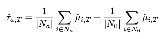
Where N_a represents the number of users in the experiment group, and N_0 represents the number of users in the control group.
There appears to be an inconsistency here: we aim to predict μ (the long-term effect of the experiment), but to train the model, we require this μ. So, how do we obtain the model? There are two approaches:
- Using pre-experiment data: We can train a model using two months of pre-experiment data for the same users.
- Similar experiments: We can select a “gold standard” experiment from the same product domain that ran for two months and use it to train the model.
In their article, Netflix validated this approach using 200 experiments and concluded that surrogate index models are consistent with long-term measurements in 95% of experiments [5].
Conclusion
We’ve learned a lot, so let’s summarize it. Short-term experiment results often differ from the long-term due to factors like heterogeneous treatment effects or user learning. There are several approaches to detect this difference, with the most straightforward being:
- Visual Approach: Simply observing the difference between the test and control over time. However, this method lacks rigor.
- Difference-in-Difference: Comparing the difference in the test and control at the beginning and after some time of the experiment.
If you suspect user learning in your experiment, the ideal approach is to extend the experiment until the treatment effect stabilizes. However, this may not always be feasible due to technical (e.g., short-lived cookies) or business restrictions. In such cases, you can predict the long-term effect using auto-surrogate models, forecasting the long-term outcome of the experiment on Y using lags of Y.
Thank you for taking the time to read this article. I would love to hear your thoughts, so please feel free to share any comments or questions you may have.
References
- N. Larsen, J. Stallrich, S. Sengupta, A. Deng, R. Kohavi, N. T. Stevens, Statistical Challenges in Online Controlled Experiments: A Review of A/B Testing Methodology (2023), https://arxiv.org/pdf/2212.11366.pdf
- S. Sadeghi, S. Gupta, S. Gramatovici, J. Lu, H. Ai, R. Zhang, Novelty and Primacy: A Long-Term Estimator for Online Experiments (2021), https://arxiv.org/pdf/2102.12893.pdf
- H. Hohnhold, D. O’Brien, D. Tang, Focusing on the Long-term: It’s Good for Users and Business (2015), https://static.googleusercontent.com/media/research.google.com/en//pubs/archive/43887.pdf
- S. Athey, R. Chetty, G. W. Imbens, H. Kang, The Surrogate Index: Combining Short-Term Proxies to Estimate Long-Term Treatment Effects More Rapidly and Precisely (2019), https://www.nber.org/system/files/working_papers/w26463/w26463.pdf
- V. Zhang, M. Zhao, A. Le, M. Dimakopoulou, N. Kallus, Evaluating the Surrogate Index as a Decision-Making Tool Using 200 A/B Tests at Netflix (2023), https://arxiv.org/pdf/2311.11922.pdf
A Guide on Estimating Long-Term Effects in A/B Tests was originally published in Towards Data Science on Medium, where people are continuing the conversation by highlighting and responding to this story.
Addressing the complexity of identifying and measuring long-term effects in online experiments

Imagine you’re an analyst at an online store. You and your team aim to understand how offering free delivery will affect the number of orders on the platform, so you decide to run an A/B test. The test group enjoys free delivery, while the control group sticks to the regular delivery fare. In the initial days of the experiment, you’ll observe more people completing orders after adding items to their carts. But the real impact is long-term — users in the test group are more likely to return for future shopping on your platform because they know you offer free delivery.
In essence, what’s the key takeaway from this example? The impact of free delivery on orders tends to increase gradually. Testing it for only a short period might mean you miss the whole story, and this is a challenge we aim to address in this article.
Understanding Why Long-Term and Short-Term Effects May Differ
Overall, there could be multiple reasons why short-term effects of the experiment differ from long-term effects [1]:
Heterogeneous Treatment Effect
- The impact of the experiment may vary for frequent and occasional users of the product. In the short run, frequent users might disproportionately influence the experiment’s outcome, introducing bias to the average treatment effect.
User Learning
- Novelty Effect — picture this: you introduce a new gamification mechanic to your product. Initially, users are curious, but this effect tends to decrease over time.
- Primacy Effect — think about when Facebook changed its ranking algorithm from chronological to recommendations. Initially, there might be a drop in time spent in the feed as users can’t find what they expect, leading to frustration. However, over time, engagement is likely to recover as users get used to the new algorithm, and discover interesting posts. Users may initially react negatively but eventually adapt, leading to increased engagement.
In this article, our focus will be on addressing two questions:
How to identify and test whether the long-term impact of the experiment differs from the short-term?
How to estimate the long-term effect when running the experiment for a sufficiently long period isn’t possible?
Methods for Identifying Trends in Long-Term Effects
Visualization
The initial step is to observe how the difference between the test and control groups changes over time. If you notice a pattern like this, you will have to dive into the details to grasp the long-term effect.
It might be also tempting to plot the experiment’s effect based not only on the experiment day but also on the number of days from the first exposure.
However, there are several pitfalls when you look at the number of days from the first exposure:
- Engaged Users Bias: The right side of the chart might show more engaged users. The observed pattern might not be due to user learning but because of diverse treatment effects. The impact on highly engaged users could be different from the effect on occasional users.
- Selective Sampling Issue: We could decide to focus solely on highly engaged users and observe how their effect evolves over time. However, this subset may not accurately represent the entire user base.
- Decreasing User Numbers: There may be only a few users who have a substantial number of days since the first exposure (the right part of the graph). This widens the confidence intervals, making it tricky to draw dependable conclusions.
The visual method for identifying long-term effects in an experiment is quite straightforward, and it’s always a good starting point to observe the difference in effects over time. However, this approach lacks rigor; you might also consider formally testing the presence of long-term effects. We’ll explore that in the next part.
Ladder Experiment Assignment [2]
The concept behind this approach is as follows: before initiating the experiment, we categorize users into k cohorts and incrementally introduce them to the experiment. For instance, if we divide users into 4 cohorts, k_1 is the control group, k_2 receives the treatment from week 1, k_3 from week 2, and k_4 from week 3.
The user-learning rate can be estimated by comparing the treatment effects from various time periods.
For instance, if you aim to estimate user learning in week 4, you would compare values T4_5 and T4_2.
The challenges with this approach are quite evident. Firstly, it introduces extra operational complexities to the experiment design. Secondly, a substantial number of users are needed to effectively divide them into different cohorts and attain reasonable statistical significance levels. Thirdly, one should anticipate having different long-term effects beforehand, and prepare to run an experiment in this complicated setting.
Difference-in-Difference [2]
This approach is a simplified version of the previous one. We split the experiment into two (or more generally, into k) time periods and compare the treatment effect in the first period with the treatment effect in the k-th period.
In this approach, a vital question is how to estimate the variance of the estimate to make conclusions about statistical significance. The authors suggest the following formula (for details, refer to the article):
σ2 — the variance of each experimental unit within each time window
ρ — the correlation of the metric for each experimental unit in two time windows
Random VS Constant Treatment Assignment³
This is another extension of the ladder experiment assignment. In this approach, the pool of users is divided into three groups: C — control group, E — the group that receives treatment throughout the experiment, and E1 — the group in which users are assigned to treatment every day with probability p. As a result, each user in the E1 group will receive treatment only a few days, preventing user learning. Now, how do we estimate user learning? Let’s introduce E1_d — a fraction of users from E1 exposed to treatment on day d. The user learning rate is then determined by the difference between E and E1_d.
User “Unlearning” [3]
This approach enables us to assess both the existence of user learning and the duration of this learning. The concept is quite elegant: it posits that users learn at the same rate as they “unlearn.” The idea is as follows: turn off the experiment and observe how the test and control groups converge over time. As both groups will receive the same treatment post-experiment, any changes in their behavior will occur because of the different treatments during the experiment period.
This approach helps us measure the period required for users to “forget” about the experiment, and we assume that this forgetting period will be equivalent to the time users take to learn during the feature roll-out.
This method has two significant drawbacks: firstly, it requires a considerable amount of time to analyze user learning. Initially, you run an experiment for an extended period to allow users to “learn,” and then you must deactivate the experiment and wait for them to “unlearn.” This process can be time-consuming. Secondly, you need to deactivate the experimental feature, which businesses may be hesitant to do.
Methods for Assessing the Long-Term Effects [4]
You’ve successfully established the existence of user learning in your experiment, and it’s clear that the long-term results are likely to differ from what you observe in the short term. Now, the question is how to predict these long-term results without running the experiment for weeks or even months.
One approach is to attempt predicting long-run outcomes of Y using short-term data. The simplest method is to use lags of Y, and it is referred to as “auto-surrogate” models. Suppose you want to predict the experiment’s result after two months but currently have only two weeks of data. In this scenario, you can train a linear regression (or any other) model:
m is the average daily outcome for user i over two months
Yi_t are value of the metric for user i at day t (T ranges from 1 to 14 in our case)
In that case, the long-term treatment effect is determined by the difference in predicted values of the metric for the test and control groups using surrogate models.
Where N_a represents the number of users in the experiment group, and N_0 represents the number of users in the control group.
There appears to be an inconsistency here: we aim to predict μ (the long-term effect of the experiment), but to train the model, we require this μ. So, how do we obtain the model? There are two approaches:
- Using pre-experiment data: We can train a model using two months of pre-experiment data for the same users.
- Similar experiments: We can select a “gold standard” experiment from the same product domain that ran for two months and use it to train the model.
In their article, Netflix validated this approach using 200 experiments and concluded that surrogate index models are consistent with long-term measurements in 95% of experiments [5].
Conclusion
We’ve learned a lot, so let’s summarize it. Short-term experiment results often differ from the long-term due to factors like heterogeneous treatment effects or user learning. There are several approaches to detect this difference, with the most straightforward being:
- Visual Approach: Simply observing the difference between the test and control over time. However, this method lacks rigor.
- Difference-in-Difference: Comparing the difference in the test and control at the beginning and after some time of the experiment.
If you suspect user learning in your experiment, the ideal approach is to extend the experiment until the treatment effect stabilizes. However, this may not always be feasible due to technical (e.g., short-lived cookies) or business restrictions. In such cases, you can predict the long-term effect using auto-surrogate models, forecasting the long-term outcome of the experiment on Y using lags of Y.
Thank you for taking the time to read this article. I would love to hear your thoughts, so please feel free to share any comments or questions you may have.
References
- N. Larsen, J. Stallrich, S. Sengupta, A. Deng, R. Kohavi, N. T. Stevens, Statistical Challenges in Online Controlled Experiments: A Review of A/B Testing Methodology (2023), https://arxiv.org/pdf/2212.11366.pdf
- S. Sadeghi, S. Gupta, S. Gramatovici, J. Lu, H. Ai, R. Zhang, Novelty and Primacy: A Long-Term Estimator for Online Experiments (2021), https://arxiv.org/pdf/2102.12893.pdf
- H. Hohnhold, D. O’Brien, D. Tang, Focusing on the Long-term: It’s Good for Users and Business (2015), https://static.googleusercontent.com/media/research.google.com/en//pubs/archive/43887.pdf
- S. Athey, R. Chetty, G. W. Imbens, H. Kang, The Surrogate Index: Combining Short-Term Proxies to Estimate Long-Term Treatment Effects More Rapidly and Precisely (2019), https://www.nber.org/system/files/working_papers/w26463/w26463.pdf
- V. Zhang, M. Zhao, A. Le, M. Dimakopoulou, N. Kallus, Evaluating the Surrogate Index as a Decision-Making Tool Using 200 A/B Tests at Netflix (2023), https://arxiv.org/pdf/2311.11922.pdf
A Guide on Estimating Long-Term Effects in A/B Tests was originally published in Towards Data Science on Medium, where people are continuing the conversation by highlighting and responding to this story.
Denial of responsibility! Techno Blender is an automatic aggregator of the all world’s media. In each content, the hyperlink to the primary source is specified. All trademarks belong to their rightful owners, all materials to their authors. If you are the owner of the content and do not want us to publish your materials, please contact us by email – [email protected]. The content will be deleted within 24 hours.