
A Sharp and Solid Outline of 3D Grid Neighborhoods
How 2D grid-based algorithms can be brought into the 3D world
In my previous two articles, A Short and Direct Walk with Pascal’s Triangle and A Quick and Clear Look at Grid-Based Visibility, we saw how easy it is to generate decent-looking travel paths and compute visible regions using grid-based algorithms. The techniques I shared in those posts can be used for video games, mobile robotics, and architectural design, though our examples were limited to two dimensions. In this third and final installment of the series, we take what we know about 2D grid-based algorithms and add the third dimension. Read on to discover five 3D grid neighborhoods you can use to solve AI problems like navigation and visibility in 3D.
3D Navigation and Visibility Problems
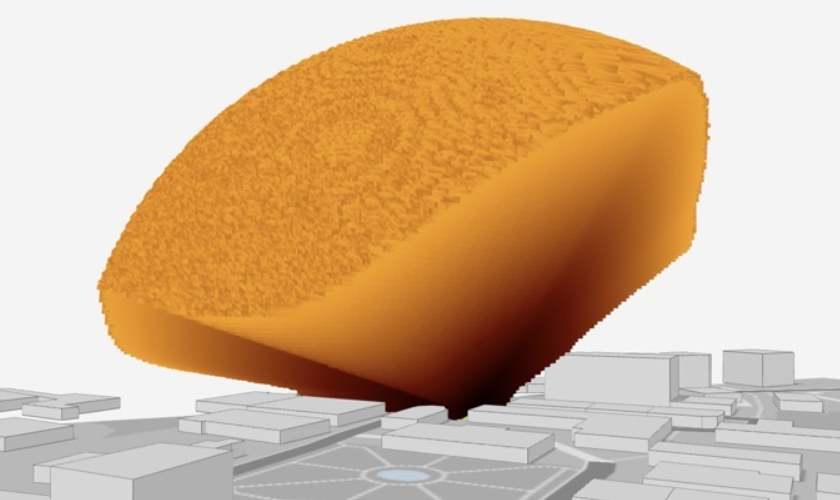
Since the world is 3D, it’s no surprise that video games, mobile robotics challenges, and architectural design tools often require 3D variants of pathfinding and visibility algorithms. For example, the image below shows what a person can see from a certain point in a 3D model of a city. An architect might use this kind of 3D visibility analysis to design a large building while allowing nearby pedestrians to see as much of the sky as possible.
This next image gives us an X-ray view of the route a person might walk between two points on different floors of a building.
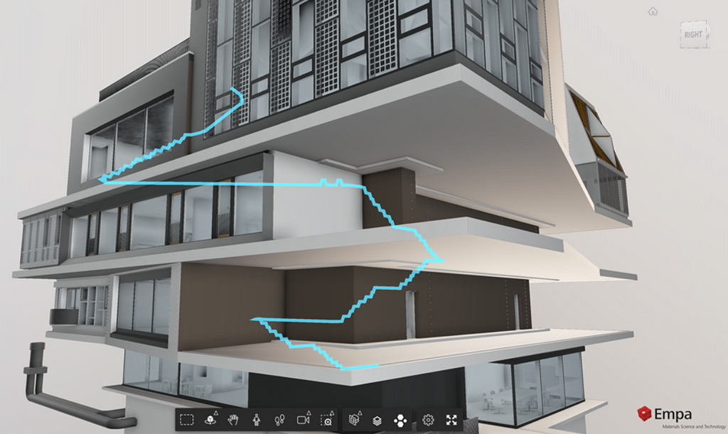
The above example is typical of 3D pathfinding in that the path is constrained to walkable surfaces such as staircases and floors. Another type of 3D navigation problem arises when generating a flight path for an aerial robot such as a quadcopter drone. In that case, the path may go straight through the air instead of adhering to surfaces.
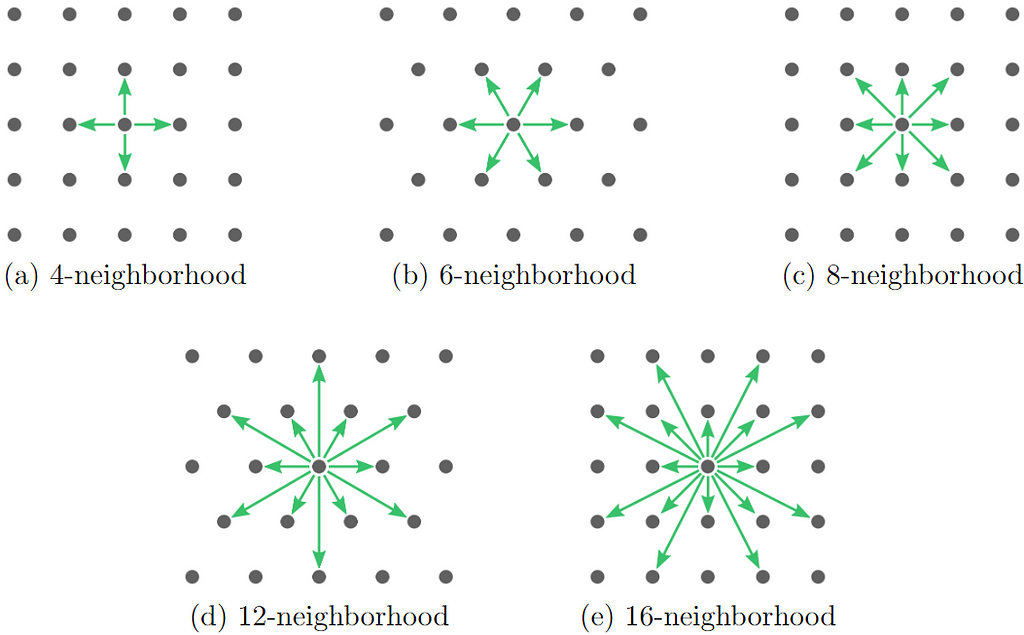
As in the previous articles, we are interested in solving navigation and visibility problems using grid-based algorithms. This means that every time a grid point is visited, information may flow only to neighboring grid points. The set of grid points considered to be “neighbors” is given by the grid neighborhood. There are many possible grid neighborhoods, but the ones depicted in the image below are the five smallest standard 2D grid neighborhoods [1]. Notice that as the neighborhoods increase in size from 4 to 16 neighbors, they alternate between rectangular and triangular grids. Generally speaking, algorithms that use larger neighborhoods take longer to run but produce more accurate results.
What interests us now is the following question:
What do these 2D neighborhoods look like in 3D?
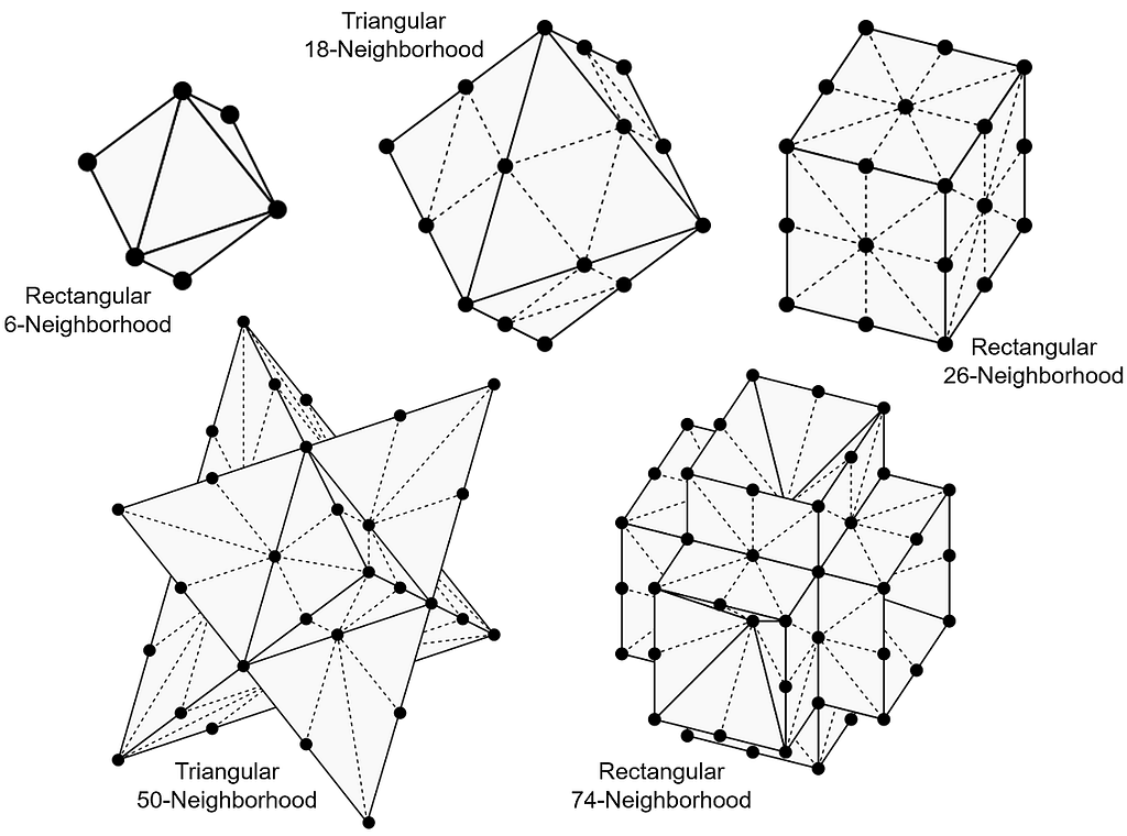
The 3D equivalent of the 4-neighborhood and the 8-neighborhood are described in the journal paper “Path Counting for Grid-Based Navigation” and elsewhere in the literature, but I had difficulty finding the 3D versions of the other three neighborhoods. I eventually decided to work them out myself so that I could present the complete set. Before we go through them one by one, here’s a sneak peek at the five smallest standard 3D grid neighborhoods.
To demonstrate these five neighborhoods, we’ll solve the 3D visibility problem with each of them and compare the five solutions for accuracy. The reason we’re focusing on grid-based visibility is because it’s one of the simplest grid-based algorithms — simple enough for us to take a good look at the code. Once you’ve seen how grid-based visibility can be implemented in 3D, you can use your choice of 3D grid neighborhood to solve 3D pathfinding problems and other AI challenges that arise in the 3D world.
Rectangular 6-Neighborhood
We’ll start with the neighborhoods defined on a 3D rectangular grid, which is simply the set of points [x, y, z] where x, y, and z are integers. These grids are widely used. They can be represented on a computer using a standard 3D array.
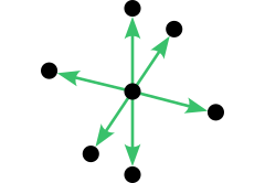
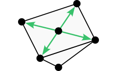
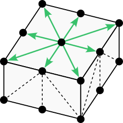
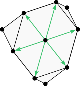
The first 3D grid neighborhood is nearly ubiquitous, but we’ll present it anyway for the sake of completeness. When the rectangular 4-neighborhood in 2D is extended to 3D, we end up with the rectangular 6-neighborhood illustrated below. To interpret the image, imagine that the two vertical arrows point up and down while the remaining arrows point north, east, south, and west.
Now we’ll apply the rectangular 6-neighborhood to solve the 3D visibility problem using Python. In the code below, the function grid_visibility inputs a 3D array named grid0 representing the environment. Cells in this initial grid with a value of 1 represent empty space, and cells with a value of 0 represent an obstacle. The function computes the visibility results in a separate 3D array named grid. Cells in this output grid with a value of 1 are considered visible from a viewpoint at [0, 0, 0], and cells with a value of 0 are considered blocked.
import numpy as np

# Solve the 3D visibility problem using a simple grid-based method
def grid_visibility(grid0):
    grid = grid0.copy()
    for x in range(grid.shape[0]):
        for y in range(grid.shape[1]):
            for z in range(int(x==0 and y==0), grid.shape[2]):
                vx = grid[x-1,y,z]
                vy = grid[x,y-1,z]
                vz = grid[x,y,z-1]
                grid[x,y,z] *= (x*vx + y*vy + z*vz) / (x + y + z)
    return grid >= 0.5
The reason the viewpoint is fixed at [0, 0, 0] is just to simplify the code. If you want the viewpoint to be located somewhere else, such as the center of the grid, the previous article solves that problem in 2D with an array indexing trick that will also work in 3D.
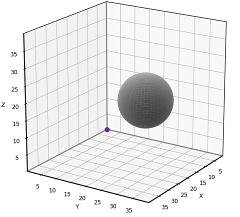
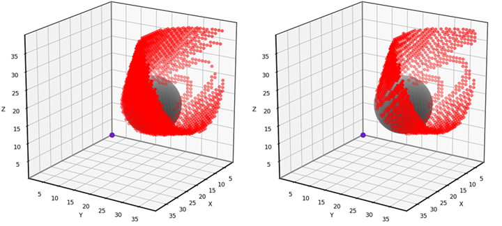
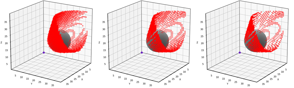
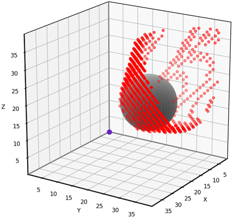
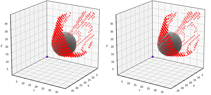
To test our 3D grid-based visibility solver, we’ll use the scenario shown below. The input grid is 40x40x40 and features a spherical obstacle with center at [10, 20, 16] and radius 8.
This problem is simple enough to solve analytically, allowing us to test the accuracy of the grid-based solution. The red dots in the animation below indicate the grid points that have been misclassified using our 6-neighbor grid-based approach. Notice that the vast majority of the 40x40x40 grid points have no red dot, meaning that they are correctly classified. The errors occur near the boundary of the obstacle’s “shadow”, where grid points are either barely visible or barely obstructed. I find that errors such as these are usually tolerable, though it depends on the application. I’ll provide the testing and visualization code near the end of the article.
Now we are going to rewrite our grid-based visibility algorithm in a way that accommodates the larger 3D grid neighborhoods. The key is to solve the visibility problem within a cone bracketed by a set of vectors. In the previous article, we defined a 2D visibility_within_cone function that required two vectors to specify a triangular cone. In 3D, the function requires three vectors to define a tetrahedral cone.
# Solve the 3D visibility problem by modifying a grid within a cone
def visibility_within_cone(grid, u_vector, v_vector, w_vector):
    u = np.asarray(u_vector, dtype=int)
    v = np.asarray(v_vector, dtype=int)
    w = np.asarray(w_vector, dtype=int)
    origin = np.array([0,0,0], dtype=int)
    dims = np.asarray(grid.shape, dtype=int)
    m = 0
    k = 0
    q = 0
    pos = np.array([0,0,0], dtype=int)
    while np.all(pos < dims):
        while np.all(pos < dims):
            while np.all(pos < dims):
                if not np.all(pos == 0):
                    p = tuple(pos)
                    if grid[p] == 1:
                        pu = tuple(np.maximum(origin, pos - u))
                        pv = tuple(np.maximum(origin, pos - v))
                        pw = tuple(np.maximum(origin, pos - w))
                        grid[p] = (m*grid[pu] +
                                   k*grid[pv] +
                                   q*grid[pw]) / (m + k + q)
                q += 1
                pos += w
            k += 1
            q = 0
            pos = m*u + k*v
        m += 1
        k = 0
        q = 0
        pos = m*u
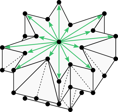
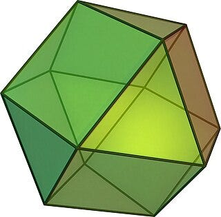
Below is an alternative illustration of the 6-neighborhood showing the triangular faces associated with each cone. Represented in this fashion, the 6-neighborhood appears as an octahedron.
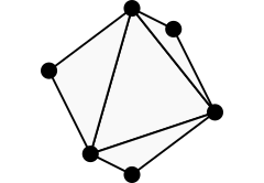
If we slice the octahedron in half, we can see the rectangular 6-neighborhood’s 2D counterpart: the 4-neighborhood.
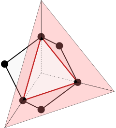
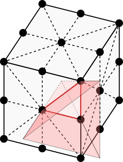
Let’s look at the full octahedron again, and project one of the triangles away from the origin to help us visualize a tetrahedral cone. The 6-neighborhood has 8 such cones in total, one for each 3D octant of the domain. Note that each cone extends to infinity, taking up its entire octant.
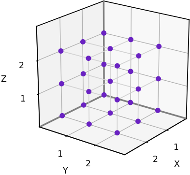
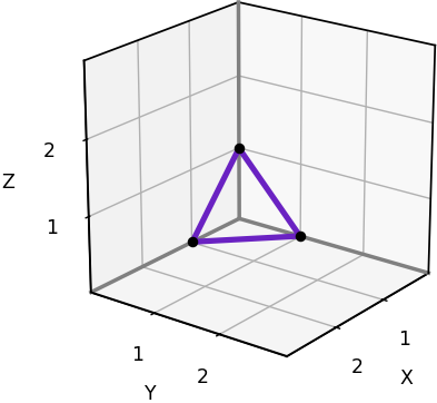
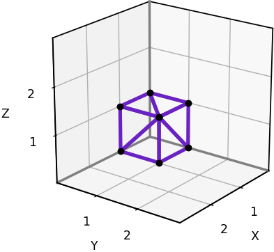
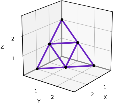
Here is a plot of just one octant of the 6-neighborhood, with its single cone. The plot makes it easy to read off the coordinates of the bracketing vectors, which we’ll need in order to reimplement the grid-based algorithm. In this case the bracketing vectors are [1,0,0], [0,1,0], [0,0,1], the corners of the triangle.
Below is our new implementation of 6-neighbor 3D grid-based visibility.
# Solve the 3D visibility problem using the 6-neighborhood
def grid6_visibility(grid0):
    grid = grid0.copy()
    visibility_within_cone(grid, [1,0,0], [0,1,0], [0,0,1])
    return grid >= 0.5
The new grid6-visibility function produces exactly the same results as the grid-visibility function we saw earlier, but our refactoring efforts will help us tackle the larger 3D neighborhoods which have many more cones.
Rectangular 26-Neighborhood
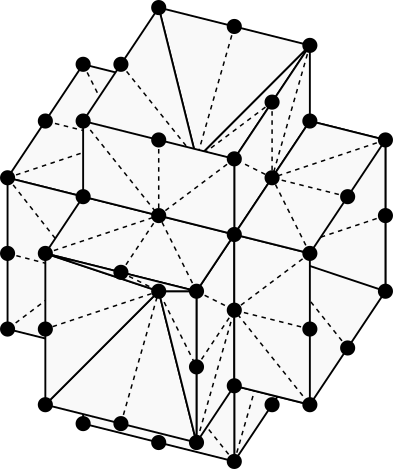
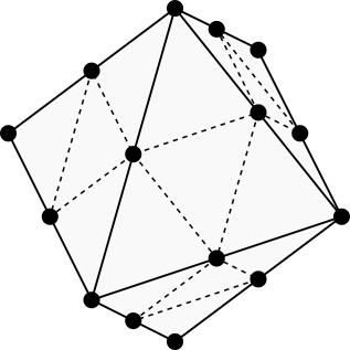
When the rectangular 8-neighborhood in 2D is extended to 3D, we get the rectangular 26-neighborhood shown below. The neighborhood appears as a 2x2x2 cube with each side tessellated into triangles representing cones.
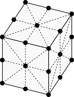
As before, we can cut the neighborhood in half to see its 2D counterpart: the 8-neighborhood.
The rectangular 26-neighborhood is well known, though it is rarely shown in a way that identifies its 48 tetrahedral cones. The illustration below highlights one of these cones.
The following plot helps us to read off the coordinates of the 6 cones within one octant.
Here’s our implementation of 26-neighbor 3D grid-based visibility. Notice that we call visibility_within_cone once for each triangle in the plot above.
# Solve the 3D visibility problem using the 26-neighborhood
def grid26_visibility(grid0):
    grid = grid0.copy()
    visibility_within_cone(grid, [1,0,0], [1,1,0], [1,1,1])
    visibility_within_cone(grid, [1,0,0], [1,0,1], [1,1,1])
    visibility_within_cone(grid, [0,1,0], [1,1,0], [1,1,1])
    visibility_within_cone(grid, [0,1,0], [0,1,1], [1,1,1])
    visibility_within_cone(grid, [0,0,1], [1,0,1], [1,1,1])
    visibility_within_cone(grid, [0,0,1], [0,1,1], [1,1,1])
    return grid >= 0.5
The visibility results we obtain with the 26-neighborhood contain fewer errors than with the 6-neighborhood. You can see below that the red dots are sparser.
The 26-neighborhood is common, though it is usually presented without identifying the 48 tetrahedral cones. In theory these cones aren’t needed for pathfinding or visibility, but they allow us to adopt faster algorithms. For example, it is widely understood among computer scientists that one can find shortest grid paths in 3D by applying Dijkstra’s algorithm using 26 neighbors on a rectangular grid. Dijkstra’s algorithm does not require us to know how those neighbors are grouped into cones. However, if we have identified the cones, we can adopt a faster pathfinding method called 3D Jump Point Search [2]. If you’re looking for a challenge, try implementing Jump Point Search with your choice of 3D grid neighborhood.
Rectangular 74-Neighborhood
The previous two 3D grid neighborhoods are reasonably well established, but now we must venture into unknown territory. When the rectangular 16-neighborhood in 2D is extended to 3D, we get the rectangular 74-neighborhood. I’m not sure how to describe the shape of the 74-neighborhood, but this is what it looks like.
And here it is again, this time sliced in half to reveal the 16-neighborhood.
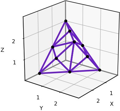
The rectangular 74-neighborhood has 144 cones in total. Below is a plot representing the 18 cones in one octant.
Reading off the coordinates of each triangle in the plot, we can now implement 74-neighbor 3D grid-based visibility.
# Solve the 3D visibility problem using the 74-neighborhood
def grid74_visibility(grid0):
    grid = grid0.copy()
    visibility_within_cone(grid, [1,0,0], [2,1,0], [2,1,1])
    visibility_within_cone(grid, [1,1,0], [2,1,0], [2,1,1])
    visibility_within_cone(grid, [1,1,0], [1,1,1], [2,1,1])
    visibility_within_cone(grid, [1,0,0], [2,0,1], [2,1,1])
    visibility_within_cone(grid, [1,0,1], [2,0,1], [2,1,1])
    visibility_within_cone(grid, [1,0,1], [1,1,1], [2,1,1])
    visibility_within_cone(grid, [0,1,0], [1,2,0], [1,2,1])
    visibility_within_cone(grid, [1,1,0], [1,2,0], [1,2,1])
    visibility_within_cone(grid, [1,1,0], [1,1,1], [1,2,1])
    visibility_within_cone(grid, [0,1,0], [0,2,1], [1,2,1])
    visibility_within_cone(grid, [0,1,1], [0,2,1], [1,2,1])
    visibility_within_cone(grid, [0,1,1], [1,1,1], [1,2,1])
    visibility_within_cone(grid, [0,0,1], [1,0,2], [1,1,2])
    visibility_within_cone(grid, [1,0,1], [1,0,2], [1,1,2])
    visibility_within_cone(grid, [1,0,1], [1,1,1], [1,1,2])
    visibility_within_cone(grid, [0,0,1], [0,1,2], [1,1,2])
    visibility_within_cone(grid, [0,1,1], [0,1,2], [1,1,2])
    visibility_within_cone(grid, [0,1,1], [1,1,1], [1,1,2])
    return grid >= 0.5
Below are the errors for all three of our 3D rectangular grid neighborhoods applied to the test scenario. The 74-neighbor solution contains the fewest misclassified points.
Triangular 18-Neighborhood
With the 3D rectangular neighborhoods taken care of, it’s time to see what the triangular neighborhoods look like in 3D. They’re surprisingly hard to visualize! A good way to start is by asking the following question:
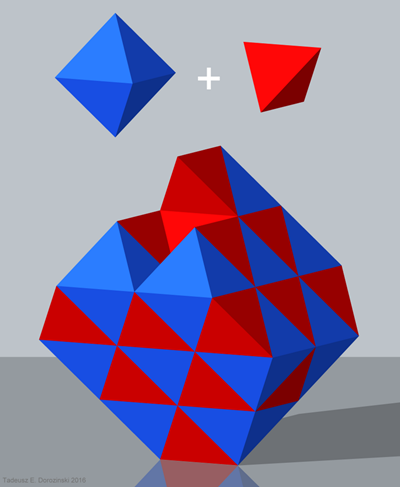
What solid objects have faces that are equilateral triangles, and can be used to fill 3D space?
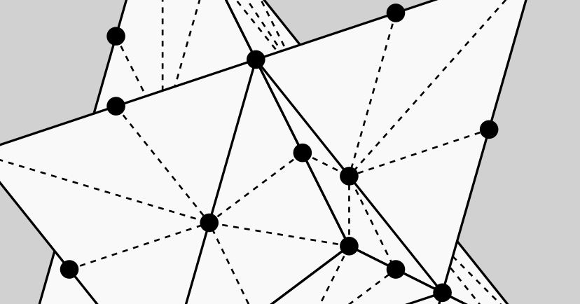
Aristotle took a stab at answering that question over 2000 years ago. He famously taught that regular tetrahedra fill space [3]. He was wrong. If you have a whole bunch of regular tetrahedra and try putting them together, you will necessarily end up with gaps. The same can be said for regular octahedra: they also do not fill space. But as shown below, you can fill space using both tetrahedra and octahedra.
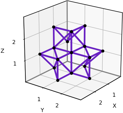
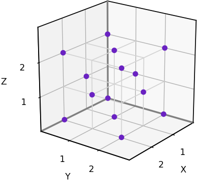
In the space-filling arrangement above, notice that the vertices of the tetrahedra and octahedra occur at regularly spaced points. These are the points of a face-centered cubic lattice, which we’ll refer to as a 3D triangular grid. If one of these points is located at [0, 0, 0], we can scale and orient the 3D triangular grid so that its points coincide with every alternate point on a 3D rectangular grid. The plot below shows a 3D triangular grid with this configuration.
To represent these grids on a computer, we’ll adopt the same kind of arrays that we employed for 3D rectangular grids. However, in the case of a 3D triangular grid, only half of the array elements will ever get used. An array element at [x, y, z] will be used only if (x + y + z) is an even number. If (x + y + z) is odd, the element will be initialized to 0 and will always remain 0.
We now know how points in a 3D triangular grid can be arranged, but what does a triangular grid cell look like in 3D? When I use the term “grid cell”, I’m referring to a space filling shape that is centered on a grid point. In 2D, a triangular grid cell is not a triangle, but rather a hexagon. The Red Blog Games tutorial on Hexagonal Grids makes this easy to see. It turns out that in 3D, a triangular grid cell is called a rhombic dodecahedron. Rhombic dodecahedra fill 3D space.
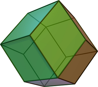
The dual of a polyhedron is the shape you get when you replace each face with a vertex and each vertex with a face. The dual of a rhombic dodecahedron is called a cuboctahedron.
If we center a cuboctahedron on a 3D triangular grid point, we can scale and orient it so that its 12 vertices coincide with the nearest neighboring grid points. In other words, the cuboctahedron is a viable 3D grid neighborhood. I would not consider this 12-neighborhood to be a standard 3D grid neighborhood, however, for the simple reason that some its faces are squares rather than triangles. There is a grid-based visibility algorithm from the urban design community that could be adapted to work with the square faces of the 12-neighborhood [4], but we will stick with our current algorithm requiring triangular faces.
The smallest 3D triangular neighborhood that meets our criteria is the triangular 18-neighborhood. It appears as an octahedron with each side tessellated into triangles.
If we slice the 18-neighborhood at an angle, we can see that it extends the 2D triangular 6-neighborhood.
The triangular 18-neighborhood has 32 cones, 4 cones per octant.
Here’s our 18-neighbor implementation of grid-based visibility.
# Solve the 3D visibility problem using the 18-neighborhood
def grid18_visibility(grid0):
    grid = grid0.copy()
    visibility_within_cone(grid, [2,0,0], [1,1,0], [1,0,1])
    visibility_within_cone(grid, [0,2,0], [1,1,0], [0,1,1])
    visibility_within_cone(grid, [0,0,2], [1,0,1], [0,1,1])
    visibility_within_cone(grid, [1,1,0], [1,0,1], [0,1,1])
    return grid >= 0.5
And here are the results.
At first glance it may seem that the 18-neighborhood has yielded greater accuracy than the three rectangular neighborhoods, even the ones with more neighbors and cones. However, the main reason the red dots are sparser here than in previous plots is because, for 3D triangular grids, we only evaluate every alternate point [x, y, z].
Triangular 50-Neighborhood
The fifth and final neighborhood in our collection is the triangular 50-neighborhood. Its overall shape is known as a stellated octahedron, which is basically an octahedron with a tetrahedron glued onto each face. In the case of the 50-neighborhood, each face of the stellated octahedron is tessellated into 4 triangles, as shown below.
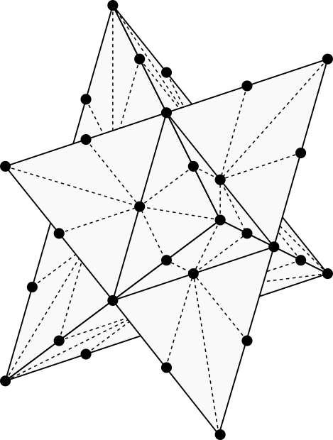
The 50-neighborhood extends the 2D triangular 12-neighborhood.
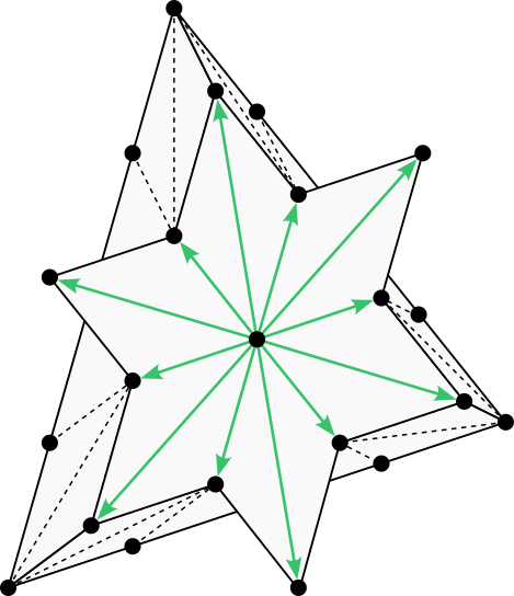
It has 96 cones, 12 per octant.
Below is 50-neighbor grid-based visibility.
# Solve the 3D visibility problem using the 50-neighborhood
def grid50_visibility(grid0):
    grid = grid0.copy()
    visibility_within_cone(grid, [2,0,0], [1,1,0], [2,1,1])
    visibility_within_cone(grid, [2,0,0], [1,0,1], [2,1,1])
    visibility_within_cone(grid, [1,1,0], [2,1,1], [2,2,2])
    visibility_within_cone(grid, [1,0,1], [2,1,1], [2,2,2])
    visibility_within_cone(grid, [0,2,0], [1,1,0], [1,2,1])
    visibility_within_cone(grid, [0,2,0], [0,1,1], [1,2,1])
    visibility_within_cone(grid, [1,1,0], [1,2,1], [2,2,2])
    visibility_within_cone(grid, [0,1,1], [1,2,1], [2,2,2])
    visibility_within_cone(grid, [0,0,2], [1,0,1], [1,1,2])
    visibility_within_cone(grid, [0,0,2], [0,1,1], [1,1,2])
    visibility_within_cone(grid, [1,0,1], [1,1,2], [2,2,2])
    visibility_within_cone(grid, [0,1,1], [1,1,2], [2,2,2])
    return grid >= 0.5
And finally, here are the results for both of our 3D triangular grid neighborhoods. It may be hard to tell at a glance, but the 50-neighbor results contain fewer errors.
Comparison of Neighborhoods
The table below lists the five presented 3D grid neighborhoods, their properties, and the accuracy obtained when applying each neighborhood to our test problem. The accuracy values are calculated by taking the number of grid points correctly classified as visible or not visible, and dividing by the total number of evaluated grid points. As we’d expect, the accuracy scores increase with the number of neighbors.
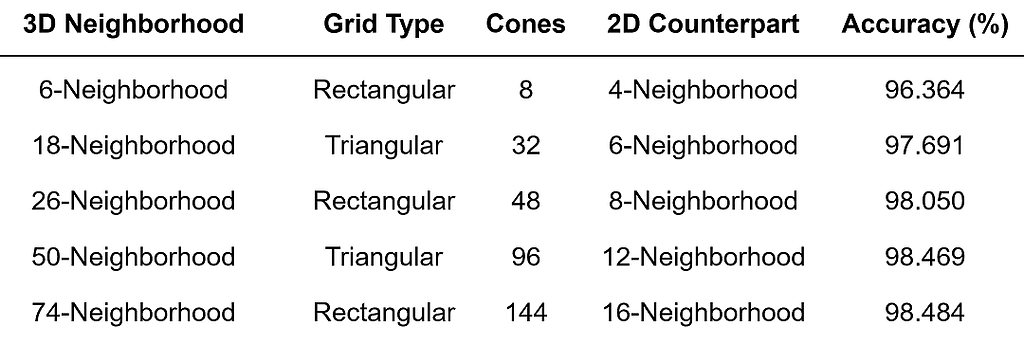
This analysis is mostly for illustrative purposes. If our goal were to perform a rigorous comparison of these five 3D grid neighborhoods, we would not be satisfied with our single test scenario. Instead we would want to apply each neighborhood to a large set of test scenarios, and average the results.
I should also point out that in this article and the previous one, I have taken a shortcut both literally and figuratively when implementing grid-based visibility for large neighborhoods. The proper formula, which you can find in the journal paper “Path Counting for Grid-Based Navigation” [1], requires a line-of-sight test between every pair of neighboring grid points. To illustrate, consider the following 2D scenario.
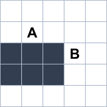
If we’re using the 4-neighborhood or the 8-neighborhood, then cells A and B in the above example are not neighbors. But if we’re using the 16-neighborhood, then these two points are neighbors and so we should technically perform a line-of-sight test between them. The algorithms in this article series alleviate the need for line-of-sight checks between distant grid points, though it is still best to precompute these checks over the short distances between neighbors. If we draw a line between the centers of cells A and B, the line will pass through a blocked cell. This suggests that the visibility algorithm should probably not propagate information directly from A to B.
The literal and figurative shortcut I’ve been taking is to assume two neighboring cells are mutually visible as long as they’re both empty. This works perfectly well for the 4-neighborhood in 2D and the 6-neighborhood in 3D, but it isn’t quite right for the larger neighborhoods. In the example above, a 16-neighbor version of my Python code would treat cells A and B as mutually visible. It would happily propagate information from one to the other, essentially taking a “shortcut” through the obstacle.
This shortcut I’m describing isn’t such a big deal if our obstacles are sufficiently wide compared with the grid spacing. In our test results, the larger 3D neighborhoods achieved greater accuracy than the smaller ones despite this flaw. But if you plan to use large 2D or 3D grid neighborhoods in your own work, I encourage you to carefully consider which neighboring grid points should and should not be treated as direct pathways for information.
Testing and Visualization Code
Please skip this section and proceed to the conclusion if you are not interested in running the Python code presented in this article.
If you are interested in running the code, follow these steps:
- Make sure you have Python installed along with the NumPy and Matplotlib libraries.
- Create an empty text file named grid_visibility_3D.py. Starting from the top, copy into this text file all of the code blocks that have appeared in this article until this point.
- Create another text file named test_grid_visibility_3D.py and copy in the long code block that appears below these instructions.
- On the command prompt, run python test_grid_visibility_3D.py. You should see the same accuracy scores that were reported in the Comparison of Neighborhoods table. You should also see a 3D visualization of the test scenario.
- Close the visualization window and run the command python test_grid_visibility_3D.py 6. You should see the same output except with red dots appearing in the 3D visualization. You can drag the cursor on the plot to rotate it and get a better view. These dots are the errors associated with the 6-neighbor visibility algorithm. Run the code again with the command line argument 6 changed to 18, 26, 50, or 74 to see the errors associated with the other 3D grid neighborhoods.
from grid_visibility_3D import *

import matplotlib.pyplot as plt
import sys

# Set dimensions for the test scenario
nx = 40
ny = 40
nz = 40

# Set spherical obstacle parameters for the test scenario
x_sphere = 10
y_sphere = 20
z_sphere = 16
r_sphere = 8

# Initialize the 3D visibility problem for the test scenario
def initial_grid():
    grid = np.ones((nx,ny,nz))
    p_sphere = np.array([x_sphere, y_sphere, z_sphere])
    for x in range(nx):
        for y in range(ny):
            for z in range(nz):
                p = np.array([x,y,z])
                r = np.sqrt(np.sum((p - p_sphere)**2))
                if r < r_sphere:
                    grid[x,y,z] = 0
    return grid

# Solve the 3D visibility problem analytically for the test scenario
def analytic_solution():
    grid = initial_grid()
    p_sphere = np.array([x_sphere, y_sphere, z_sphere])
    d_sphere = np.sqrt(np.sum(p_sphere**2))
    u = p_sphere/d_sphere
    for x in range(nx):
        for y in range(ny):
            for z in range(nz):
                if grid[x,y,z]:
                    p = np.array([x,y,z])
                    d = np.sum(p*u)
                    if d > d_sphere:
                        h = np.sqrt(np.sum((p - d*u)**2))
                        grid[x,y,z] = h*d_sphere >= d*r_sphere
    return grid

# Compare the 3D grid-based results to the analytic solution
def evaluate_grid(test_name, grid, solution, triangular=False):
    error_grid = np.abs(grid - solution)
    total_count = nx*ny*nz
    if triangular:
        for x in range(nx):
            for y in range(ny):
                for z in range(nz):
                    if (x + y + z)%2 == 1:
                        error_grid[x,y,z] = 0
                        total_count -= 1
    error_count = int(np.sum(error_grid))
    accuracy = 100*(1 - error_count/total_count)
    print(test_name + " accuracy: %.3f" % accuracy)
    return error_grid

# Plot the 3D visibility problem with or without resulting errors
def plot_test_scenario(error_grid=None, obstacle=True, pretty=True):
    elevation = 19
    azimuth = 33
    ax = plt.figure().add_subplot(projection='3d')
    ax.view_init(elev=elevation, azim=azimuth, roll=0)
    ax.set_aspect('equal')
    ax.set_xlabel('X')
    ax.set_ylabel('Y')
    ax.set_zlabel('Z')
    ax.scatter(0, 0, 0, color='#6A22C2', s=64)  # Render viewpoint
    if pretty:
        # Choose limits that avoid padding
        ax.set_xlim(0.9, nx - 0.9)
        ax.set_ylim(0.9, ny - 0.9)
        ax.set_zlim(0.9, nz - 0.9)
        # Ensure axes are prominently displayed
        ax.plot([0,nx], [0,0], [0,0], color='gray', linewidth=2)
        ax.plot([0,nx], [ny,ny], [0,0], color='black', linewidth=1)
        ax.plot([0,nx], [0, 0], [nz,nz], color='black', linewidth=1)
        ax.plot([0,0], [0,ny], [0,0], color='gray', linewidth=2)
        ax.plot([nx,nx], [0,ny], [0,0], color='black', linewidth=1)
        ax.plot([0,0], [0,ny], [nz,nz], color='black', linewidth=1)
        ax.plot([0,0], [0,0], [0,nz], color='gray', linewidth=2)
        ax.plot([0,0], [ny,ny], [0,nz], color='black', linewidth=1)
        ax.plot([nx,nx], [0,0], [0,nz], color='black', linewidth=1)
    else:
        ax.set_xlim(0, nx)
        ax.set_ylim(0, ny)
        ax.set_zlim(0, nz)
    if obstacle:
        n = 100
        us = np.linspace(0, 2*np.pi, n)
        vs = np.linspace(0, np.pi, n)
        xs = r_sphere*np.outer(np.cos(us), np.sin(vs)) + x_sphere
        ys = r_sphere*np.outer(np.sin(us), np.sin(vs)) + y_sphere
        zs = r_sphere*np.outer(np.ones(n), np.cos(vs)) + z_sphere
        ax.plot_surface(xs, ys, zs, color='lightgray')
    if np.all(error_grid) != None:
        error_count = int(np.sum(error_grid))
        xs = np.zeros(error_count)
        ys = np.zeros(error_count)
        zs = np.zeros(error_count)
        i = 0
        for x in range(nx):
            for y in range(ny):
                for z in range(nz):
                    if error_grid[x,y,z]:
                        xs[i] = x
                        ys[i] = y
                        zs[i] = z
                        i += 1
        ax.scatter(xs, ys, zs, color='red')
    plt.show()

if __name__ == "__main__":
    # Compute the grid-based solutions
    grid0 = initial_grid()
    grid = grid_visibility(grid0)
    grid6 = grid6_visibility(grid0)
    grid18 = grid18_visibility(grid0)
    grid26 = grid26_visibility(grid0)
    grid50 = grid50_visibility(grid0)
    grid74 = grid74_visibility(grid0)
    # Ensure that 6-neighbor solutions are identical
    if np.any(grid != grid6):
        print("Warning: Alternative 6-neighbor solutions differ")
    # Compute the analytic solution
    solution = analytic_solution()
    # Compute the errors and report accuracy
    error_grid6 = evaluate_grid(' 6-neighbor', grid6, solution)
    error_grid18 = evaluate_grid('18-neighbor', grid18, solution, True)
    error_grid26 = evaluate_grid('26-neighbor', grid26, solution)
    error_grid50 = evaluate_grid('50-neighbor', grid50, solution, True)
    error_grid74 = evaluate_grid('74-neighbor', grid74, solution)
    # Plot the results
    error_grid = None
    if len(sys.argv) >= 2:
        if sys.argv[1] == "6":
            error_grid = error_grid6
        elif sys.argv[1] == "18":
            error_grid = error_grid18
        elif sys.argv[1] == "26":
            error_grid = error_grid26
        elif sys.argv[1] == "50":
            error_grid = error_grid50
        elif sys.argv[1] == "74":
            error_grid = error_grid74
    plot_test_scenario(error_grid)
Conclusion
Thank you for reading my articles on pathfinding and visibility in both 2D and 3D. I hope this series has expanded your view of what can be done using simple grid-based algorithms. By counting paths (see part 1), employing linear interpolation (see part 2), selecting a larger grid neighborhood (as in this article — part 3), or simply choosing a finer grid resolution, we can overcome the perceived limitations of grids and achieve highly satisfactory results. The next time you encounter an AI problem that is usually tackled with brute force ray casting or cumbersome analytic calculations, remember what you can accomplish with a grid-based method and your neighborhood of choice.
References
[1] R. Goldstein, K. Walmsley, J. Bibliowicz, A. Tessier, S. Breslav, A. Khan, Path Counting for Grid-Based Navigation (2022), Journal of Artificial Intelligence Research, vol. 74, pp. 917–955
[2] T. K. Nobes, D. D. Harabor, M. Wybrow, S. D. C. Walsh, The Jump Point Search Pathfinding System in 3D (2022), Proceedings of the International Symposium on Combinatorial Search (SoCS)
[3] C. L. Jeffrey, C. Zong, Mysteries in Packing Regular Tetrahedra (2012), Notices of the American Mathematical Society, vol. 59, no. 11, pp. 1540–1549
[4] D. Fisher-Gewirtzman, A. Shashkov, Y. Doytsher, Voxel Based Volumetric Visibility Analysis of Urban Environments (2013), Survey Review, vol. 45, no. 333, pp. 451–461
A Sharp and Solid Outline of 3D Grid Neighborhoods was originally published in Towards Data Science on Medium, where people are continuing the conversation by highlighting and responding to this story.
How 2D grid-based algorithms can be brought into the 3D world
In my previous two articles, A Short and Direct Walk with Pascal’s Triangle and A Quick and Clear Look at Grid-Based Visibility, we saw how easy it is to generate decent-looking travel paths and compute visible regions using grid-based algorithms. The techniques I shared in those posts can be used for video games, mobile robotics, and architectural design, though our examples were limited to two dimensions. In this third and final installment of the series, we take what we know about 2D grid-based algorithms and add the third dimension. Read on to discover five 3D grid neighborhoods you can use to solve AI problems like navigation and visibility in 3D.
3D Navigation and Visibility Problems
Since the world is 3D, it’s no surprise that video games, mobile robotics challenges, and architectural design tools often require 3D variants of pathfinding and visibility algorithms. For example, the image below shows what a person can see from a certain point in a 3D model of a city. An architect might use this kind of 3D visibility analysis to design a large building while allowing nearby pedestrians to see as much of the sky as possible.
This next image gives us an X-ray view of the route a person might walk between two points on different floors of a building.
The above example is typical of 3D pathfinding in that the path is constrained to walkable surfaces such as staircases and floors. Another type of 3D navigation problem arises when generating a flight path for an aerial robot such as a quadcopter drone. In that case, the path may go straight through the air instead of adhering to surfaces.
As in the previous articles, we are interested in solving navigation and visibility problems using grid-based algorithms. This means that every time a grid point is visited, information may flow only to neighboring grid points. The set of grid points considered to be “neighbors” is given by the grid neighborhood. There are many possible grid neighborhoods, but the ones depicted in the image below are the five smallest standard 2D grid neighborhoods [1]. Notice that as the neighborhoods increase in size from 4 to 16 neighbors, they alternate between rectangular and triangular grids. Generally speaking, algorithms that use larger neighborhoods take longer to run but produce more accurate results.
What interests us now is the following question:
What do these 2D neighborhoods look like in 3D?
The 3D equivalent of the 4-neighborhood and the 8-neighborhood are described in the journal paper “Path Counting for Grid-Based Navigation” and elsewhere in the literature, but I had difficulty finding the 3D versions of the other three neighborhoods. I eventually decided to work them out myself so that I could present the complete set. Before we go through them one by one, here’s a sneak peek at the five smallest standard 3D grid neighborhoods.
To demonstrate these five neighborhoods, we’ll solve the 3D visibility problem with each of them and compare the five solutions for accuracy. The reason we’re focusing on grid-based visibility is because it’s one of the simplest grid-based algorithms — simple enough for us to take a good look at the code. Once you’ve seen how grid-based visibility can be implemented in 3D, you can use your choice of 3D grid neighborhood to solve 3D pathfinding problems and other AI challenges that arise in the 3D world.
Rectangular 6-Neighborhood
We’ll start with the neighborhoods defined on a 3D rectangular grid, which is simply the set of points [x, y, z] where x, y, and z are integers. These grids are widely used. They can be represented on a computer using a standard 3D array.
The first 3D grid neighborhood is nearly ubiquitous, but we’ll present it anyway for the sake of completeness. When the rectangular 4-neighborhood in 2D is extended to 3D, we end up with the rectangular 6-neighborhood illustrated below. To interpret the image, imagine that the two vertical arrows point up and down while the remaining arrows point north, east, south, and west.
Now we’ll apply the rectangular 6-neighborhood to solve the 3D visibility problem using Python. In the code below, the function grid_visibility inputs a 3D array named grid0 representing the environment. Cells in this initial grid with a value of 1 represent empty space, and cells with a value of 0 represent an obstacle. The function computes the visibility results in a separate 3D array named grid. Cells in this output grid with a value of 1 are considered visible from a viewpoint at [0, 0, 0], and cells with a value of 0 are considered blocked.
import numpy as np

# Solve the 3D visibility problem using a simple grid-based method
def grid_visibility(grid0):
    grid = grid0.copy()
    for x in range(grid.shape[0]):
        for y in range(grid.shape[1]):
            for z in range(int(x==0 and y==0), grid.shape[2]):
                vx = grid[x-1,y,z]
                vy = grid[x,y-1,z]
                vz = grid[x,y,z-1]
                grid[x,y,z] *= (x*vx + y*vy + z*vz) / (x + y + z)
    return grid >= 0.5
The reason the viewpoint is fixed at [0, 0, 0] is just to simplify the code. If you want the viewpoint to be located somewhere else, such as the center of the grid, the previous article solves that problem in 2D with an array indexing trick that will also work in 3D.
To test our 3D grid-based visibility solver, we’ll use the scenario shown below. The input grid is 40x40x40 and features a spherical obstacle with center at [10, 20, 16] and radius 8.
This problem is simple enough to solve analytically, allowing us to test the accuracy of the grid-based solution. The red dots in the animation below indicate the grid points that have been misclassified using our 6-neighbor grid-based approach. Notice that the vast majority of the 40x40x40 grid points have no red dot, meaning that they are correctly classified. The errors occur near the boundary of the obstacle’s “shadow”, where grid points are either barely visible or barely obstructed. I find that errors such as these are usually tolerable, though it depends on the application. I’ll provide the testing and visualization code near the end of the article.
Now we are going to rewrite our grid-based visibility algorithm in a way that accommodates the larger 3D grid neighborhoods. The key is to solve the visibility problem within a cone bracketed by a set of vectors. In the previous article, we defined a 2D visibility_within_cone function that required two vectors to specify a triangular cone. In 3D, the function requires three vectors to define a tetrahedral cone.
# Solve the 3D visibility problem by modifying a grid within a cone
def visibility_within_cone(grid, u_vector, v_vector, w_vector):
    u = np.asarray(u_vector, dtype=int)
    v = np.asarray(v_vector, dtype=int)
    w = np.asarray(w_vector, dtype=int)
    origin = np.array([0,0,0], dtype=int)
    dims = np.asarray(grid.shape, dtype=int)
    m = 0
    k = 0
    q = 0
    pos = np.array([0,0,0], dtype=int)
    while np.all(pos < dims):
        while np.all(pos < dims):
            while np.all(pos < dims):
                if not np.all(pos == 0):
                    p = tuple(pos)
                    if grid[p] == 1:
                        pu = tuple(np.maximum(origin, pos - u))
                        pv = tuple(np.maximum(origin, pos - v))
                        pw = tuple(np.maximum(origin, pos - w))
                        grid[p] = (m*grid[pu] +
                                   k*grid[pv] +
                                   q*grid[pw]) / (m + k + q)
                q += 1
                pos += w
            k += 1
            q = 0
            pos = m*u + k*v
        m += 1
        k = 0
        q = 0
        pos = m*u
Below is an alternative illustration of the 6-neighborhood showing the triangular faces associated with each cone. Represented in this fashion, the 6-neighborhood appears as an octahedron.
If we slice the octahedron in half, we can see the rectangular 6-neighborhood’s 2D counterpart: the 4-neighborhood.
Let’s look at the full octahedron again, and project one of the triangles away from the origin to help us visualize a tetrahedral cone. The 6-neighborhood has 8 such cones in total, one for each 3D octant of the domain. Note that each cone extends to infinity, taking up its entire octant.
Here is a plot of just one octant of the 6-neighborhood, with its single cone. The plot makes it easy to read off the coordinates of the bracketing vectors, which we’ll need in order to reimplement the grid-based algorithm. In this case the bracketing vectors are [1,0,0], [0,1,0], [0,0,1], the corners of the triangle.
Below is our new implementation of 6-neighbor 3D grid-based visibility.
# Solve the 3D visibility problem using the 6-neighborhood
def grid6_visibility(grid0):
    grid = grid0.copy()
    visibility_within_cone(grid, [1,0,0], [0,1,0], [0,0,1])
    return grid >= 0.5
The new grid6-visibility function produces exactly the same results as the grid-visibility function we saw earlier, but our refactoring efforts will help us tackle the larger 3D neighborhoods which have many more cones.
Rectangular 26-Neighborhood
When the rectangular 8-neighborhood in 2D is extended to 3D, we get the rectangular 26-neighborhood shown below. The neighborhood appears as a 2x2x2 cube with each side tessellated into triangles representing cones.
As before, we can cut the neighborhood in half to see its 2D counterpart: the 8-neighborhood.
The rectangular 26-neighborhood is well known, though it is rarely shown in a way that identifies its 48 tetrahedral cones. The illustration below highlights one of these cones.
The following plot helps us to read off the coordinates of the 6 cones within one octant.
Here’s our implementation of 26-neighbor 3D grid-based visibility. Notice that we call visibility_within_cone once for each triangle in the plot above.
# Solve the 3D visibility problem using the 26-neighborhood
def grid26_visibility(grid0):
    grid = grid0.copy()
    visibility_within_cone(grid, [1,0,0], [1,1,0], [1,1,1])
    visibility_within_cone(grid, [1,0,0], [1,0,1], [1,1,1])
    visibility_within_cone(grid, [0,1,0], [1,1,0], [1,1,1])
    visibility_within_cone(grid, [0,1,0], [0,1,1], [1,1,1])
    visibility_within_cone(grid, [0,0,1], [1,0,1], [1,1,1])
    visibility_within_cone(grid, [0,0,1], [0,1,1], [1,1,1])
    return grid >= 0.5
The visibility results we obtain with the 26-neighborhood contain fewer errors than with the 6-neighborhood. You can see below that the red dots are sparser.
The 26-neighborhood is common, though it is usually presented without identifying the 48 tetrahedral cones. In theory these cones aren’t needed for pathfinding or visibility, but they allow us to adopt faster algorithms. For example, it is widely understood among computer scientists that one can find shortest grid paths in 3D by applying Dijkstra’s algorithm using 26 neighbors on a rectangular grid. Dijkstra’s algorithm does not require us to know how those neighbors are grouped into cones. However, if we have identified the cones, we can adopt a faster pathfinding method called 3D Jump Point Search [2]. If you’re looking for a challenge, try implementing Jump Point Search with your choice of 3D grid neighborhood.
Rectangular 74-Neighborhood
The previous two 3D grid neighborhoods are reasonably well established, but now we must venture into unknown territory. When the rectangular 16-neighborhood in 2D is extended to 3D, we get the rectangular 74-neighborhood. I’m not sure how to describe the shape of the 74-neighborhood, but this is what it looks like.
And here it is again, this time sliced in half to reveal the 16-neighborhood.
The rectangular 74-neighborhood has 144 cones in total. Below is a plot representing the 18 cones in one octant.
Reading off the coordinates of each triangle in the plot, we can now implement 74-neighbor 3D grid-based visibility.
# Solve the 3D visibility problem using the 74-neighborhood
def grid74_visibility(grid0):
    grid = grid0.copy()
    visibility_within_cone(grid, [1,0,0], [2,1,0], [2,1,1])
    visibility_within_cone(grid, [1,1,0], [2,1,0], [2,1,1])
    visibility_within_cone(grid, [1,1,0], [1,1,1], [2,1,1])
    visibility_within_cone(grid, [1,0,0], [2,0,1], [2,1,1])
    visibility_within_cone(grid, [1,0,1], [2,0,1], [2,1,1])
    visibility_within_cone(grid, [1,0,1], [1,1,1], [2,1,1])
    visibility_within_cone(grid, [0,1,0], [1,2,0], [1,2,1])
    visibility_within_cone(grid, [1,1,0], [1,2,0], [1,2,1])
    visibility_within_cone(grid, [1,1,0], [1,1,1], [1,2,1])
    visibility_within_cone(grid, [0,1,0], [0,2,1], [1,2,1])
    visibility_within_cone(grid, [0,1,1], [0,2,1], [1,2,1])
    visibility_within_cone(grid, [0,1,1], [1,1,1], [1,2,1])
    visibility_within_cone(grid, [0,0,1], [1,0,2], [1,1,2])
    visibility_within_cone(grid, [1,0,1], [1,0,2], [1,1,2])
    visibility_within_cone(grid, [1,0,1], [1,1,1], [1,1,2])
    visibility_within_cone(grid, [0,0,1], [0,1,2], [1,1,2])
    visibility_within_cone(grid, [0,1,1], [0,1,2], [1,1,2])
    visibility_within_cone(grid, [0,1,1], [1,1,1], [1,1,2])
    return grid >= 0.5
Below are the errors for all three of our 3D rectangular grid neighborhoods applied to the test scenario. The 74-neighbor solution contains the fewest misclassified points.
Triangular 18-Neighborhood
With the 3D rectangular neighborhoods taken care of, it’s time to see what the triangular neighborhoods look like in 3D. They’re surprisingly hard to visualize! A good way to start is by asking the following question:
What solid objects have faces that are equilateral triangles, and can be used to fill 3D space?
Aristotle took a stab at answering that question over 2000 years ago. He famously taught that regular tetrahedra fill space [3]. He was wrong. If you have a whole bunch of regular tetrahedra and try putting them together, you will necessarily end up with gaps. The same can be said for regular octahedra: they also do not fill space. But as shown below, you can fill space using both tetrahedra and octahedra.
In the space-filling arrangement above, notice that the vertices of the tetrahedra and octahedra occur at regularly spaced points. These are the points of a face-centered cubic lattice, which we’ll refer to as a 3D triangular grid. If one of these points is located at [0, 0, 0], we can scale and orient the 3D triangular grid so that its points coincide with every alternate point on a 3D rectangular grid. The plot below shows a 3D triangular grid with this configuration.
To represent these grids on a computer, we’ll adopt the same kind of arrays that we employed for 3D rectangular grids. However, in the case of a 3D triangular grid, only half of the array elements will ever get used. An array element at [x, y, z] will be used only if (x + y + z) is an even number. If (x + y + z) is odd, the element will be initialized to 0 and will always remain 0.
We now know how points in a 3D triangular grid can be arranged, but what does a triangular grid cell look like in 3D? When I use the term “grid cell”, I’m referring to a space filling shape that is centered on a grid point. In 2D, a triangular grid cell is not a triangle, but rather a hexagon. The Red Blog Games tutorial on Hexagonal Grids makes this easy to see. It turns out that in 3D, a triangular grid cell is called a rhombic dodecahedron. Rhombic dodecahedra fill 3D space.
The dual of a polyhedron is the shape you get when you replace each face with a vertex and each vertex with a face. The dual of a rhombic dodecahedron is called a cuboctahedron.
If we center a cuboctahedron on a 3D triangular grid point, we can scale and orient it so that its 12 vertices coincide with the nearest neighboring grid points. In other words, the cuboctahedron is a viable 3D grid neighborhood. I would not consider this 12-neighborhood to be a standard 3D grid neighborhood, however, for the simple reason that some its faces are squares rather than triangles. There is a grid-based visibility algorithm from the urban design community that could be adapted to work with the square faces of the 12-neighborhood [4], but we will stick with our current algorithm requiring triangular faces.
The smallest 3D triangular neighborhood that meets our criteria is the triangular 18-neighborhood. It appears as an octahedron with each side tessellated into triangles.
If we slice the 18-neighborhood at an angle, we can see that it extends the 2D triangular 6-neighborhood.
The triangular 18-neighborhood has 32 cones, 4 cones per octant.
Here’s our 18-neighbor implementation of grid-based visibility.
# Solve the 3D visibility problem using the 18-neighborhood
def grid18_visibility(grid0):
    grid = grid0.copy()
    visibility_within_cone(grid, [2,0,0], [1,1,0], [1,0,1])
    visibility_within_cone(grid, [0,2,0], [1,1,0], [0,1,1])
    visibility_within_cone(grid, [0,0,2], [1,0,1], [0,1,1])
    visibility_within_cone(grid, [1,1,0], [1,0,1], [0,1,1])
    return grid >= 0.5
And here are the results.
At first glance it may seem that the 18-neighborhood has yielded greater accuracy than the three rectangular neighborhoods, even the ones with more neighbors and cones. However, the main reason the red dots are sparser here than in previous plots is because, for 3D triangular grids, we only evaluate every alternate point [x, y, z].
Triangular 50-Neighborhood
The fifth and final neighborhood in our collection is the triangular 50-neighborhood. Its overall shape is known as a stellated octahedron, which is basically an octahedron with a tetrahedron glued onto each face. In the case of the 50-neighborhood, each face of the stellated octahedron is tessellated into 4 triangles, as shown below.
The 50-neighborhood extends the 2D triangular 12-neighborhood.
It has 96 cones, 12 per octant.
Below is 50-neighbor grid-based visibility.
# Solve the 3D visibility problem using the 50-neighborhood
def grid50_visibility(grid0):
    grid = grid0.copy()
    visibility_within_cone(grid, [2,0,0], [1,1,0], [2,1,1])
    visibility_within_cone(grid, [2,0,0], [1,0,1], [2,1,1])
    visibility_within_cone(grid, [1,1,0], [2,1,1], [2,2,2])
    visibility_within_cone(grid, [1,0,1], [2,1,1], [2,2,2])
    visibility_within_cone(grid, [0,2,0], [1,1,0], [1,2,1])
    visibility_within_cone(grid, [0,2,0], [0,1,1], [1,2,1])
    visibility_within_cone(grid, [1,1,0], [1,2,1], [2,2,2])
    visibility_within_cone(grid, [0,1,1], [1,2,1], [2,2,2])
    visibility_within_cone(grid, [0,0,2], [1,0,1], [1,1,2])
    visibility_within_cone(grid, [0,0,2], [0,1,1], [1,1,2])
    visibility_within_cone(grid, [1,0,1], [1,1,2], [2,2,2])
    visibility_within_cone(grid, [0,1,1], [1,1,2], [2,2,2])
    return grid >= 0.5
And finally, here are the results for both of our 3D triangular grid neighborhoods. It may be hard to tell at a glance, but the 50-neighbor results contain fewer errors.
Comparison of Neighborhoods
The table below lists the five presented 3D grid neighborhoods, their properties, and the accuracy obtained when applying each neighborhood to our test problem. The accuracy values are calculated by taking the number of grid points correctly classified as visible or not visible, and dividing by the total number of evaluated grid points. As we’d expect, the accuracy scores increase with the number of neighbors.
This analysis is mostly for illustrative purposes. If our goal were to perform a rigorous comparison of these five 3D grid neighborhoods, we would not be satisfied with our single test scenario. Instead we would want to apply each neighborhood to a large set of test scenarios, and average the results.
I should also point out that in this article and the previous one, I have taken a shortcut both literally and figuratively when implementing grid-based visibility for large neighborhoods. The proper formula, which you can find in the journal paper “Path Counting for Grid-Based Navigation” [1], requires a line-of-sight test between every pair of neighboring grid points. To illustrate, consider the following 2D scenario.
If we’re using the 4-neighborhood or the 8-neighborhood, then cells A and B in the above example are not neighbors. But if we’re using the 16-neighborhood, then these two points are neighbors and so we should technically perform a line-of-sight test between them. The algorithms in this article series alleviate the need for line-of-sight checks between distant grid points, though it is still best to precompute these checks over the short distances between neighbors. If we draw a line between the centers of cells A and B, the line will pass through a blocked cell. This suggests that the visibility algorithm should probably not propagate information directly from A to B.
The literal and figurative shortcut I’ve been taking is to assume two neighboring cells are mutually visible as long as they’re both empty. This works perfectly well for the 4-neighborhood in 2D and the 6-neighborhood in 3D, but it isn’t quite right for the larger neighborhoods. In the example above, a 16-neighbor version of my Python code would treat cells A and B as mutually visible. It would happily propagate information from one to the other, essentially taking a “shortcut” through the obstacle.
This shortcut I’m describing isn’t such a big deal if our obstacles are sufficiently wide compared with the grid spacing. In our test results, the larger 3D neighborhoods achieved greater accuracy than the smaller ones despite this flaw. But if you plan to use large 2D or 3D grid neighborhoods in your own work, I encourage you to carefully consider which neighboring grid points should and should not be treated as direct pathways for information.
Testing and Visualization Code
Please skip this section and proceed to the conclusion if you are not interested in running the Python code presented in this article.
If you are interested in running the code, follow these steps:
- Make sure you have Python installed along with the NumPy and Matplotlib libraries.
- Create an empty text file named grid_visibility_3D.py. Starting from the top, copy into this text file all of the code blocks that have appeared in this article until this point.
- Create another text file named test_grid_visibility_3D.py and copy in the long code block that appears below these instructions.
- On the command prompt, run python test_grid_visibility_3D.py. You should see the same accuracy scores that were reported in the Comparison of Neighborhoods table. You should also see a 3D visualization of the test scenario.
- Close the visualization window and run the command python test_grid_visibility_3D.py 6. You should see the same output except with red dots appearing in the 3D visualization. You can drag the cursor on the plot to rotate it and get a better view. These dots are the errors associated with the 6-neighbor visibility algorithm. Run the code again with the command line argument 6 changed to 18, 26, 50, or 74 to see the errors associated with the other 3D grid neighborhoods.
from grid_visibility_3D import *

import matplotlib.pyplot as plt
import sys

# Set dimensions for the test scenario
nx = 40
ny = 40
nz = 40

# Set spherical obstacle parameters for the test scenario
x_sphere = 10
y_sphere = 20
z_sphere = 16
r_sphere = 8

# Initialize the 3D visibility problem for the test scenario
def initial_grid():
    grid = np.ones((nx,ny,nz))
    p_sphere = np.array([x_sphere, y_sphere, z_sphere])
    for x in range(nx):
        for y in range(ny):
            for z in range(nz):
                p = np.array([x,y,z])
                r = np.sqrt(np.sum((p - p_sphere)**2))
                if r < r_sphere:
                    grid[x,y,z] = 0
    return grid

# Solve the 3D visibility problem analytically for the test scenario
def analytic_solution():
    grid = initial_grid()
    p_sphere = np.array([x_sphere, y_sphere, z_sphere])
    d_sphere = np.sqrt(np.sum(p_sphere**2))
    u = p_sphere/d_sphere
    for x in range(nx):
        for y in range(ny):
            for z in range(nz):
                if grid[x,y,z]:
                    p = np.array([x,y,z])
                    d = np.sum(p*u)
                    if d > d_sphere:
                        h = np.sqrt(np.sum((p - d*u)**2))
                        grid[x,y,z] = h*d_sphere >= d*r_sphere
    return grid

# Compare the 3D grid-based results to the analytic solution
def evaluate_grid(test_name, grid, solution, triangular=False):
    error_grid = np.abs(grid - solution)
    total_count = nx*ny*nz
    if triangular:
        for x in range(nx):
            for y in range(ny):
                for z in range(nz):
                    if (x + y + z)%2 == 1:
                        error_grid[x,y,z] = 0
                        total_count -= 1
    error_count = int(np.sum(error_grid))
    accuracy = 100*(1 - error_count/total_count)
    print(test_name + " accuracy: %.3f" % accuracy)
    return error_grid

# Plot the 3D visibility problem with or without resulting errors
def plot_test_scenario(error_grid=None, obstacle=True, pretty=True):
    elevation = 19
    azimuth = 33
    ax = plt.figure().add_subplot(projection='3d')
    ax.view_init(elev=elevation, azim=azimuth, roll=0)
    ax.set_aspect('equal')
    ax.set_xlabel('X')
    ax.set_ylabel('Y')
    ax.set_zlabel('Z')
    ax.scatter(0, 0, 0, color='#6A22C2', s=64)  # Render viewpoint
    if pretty:
        # Choose limits that avoid padding
        ax.set_xlim(0.9, nx - 0.9)
        ax.set_ylim(0.9, ny - 0.9)
        ax.set_zlim(0.9, nz - 0.9)
        # Ensure axes are prominently displayed
        ax.plot([0,nx], [0,0], [0,0], color='gray', linewidth=2)
        ax.plot([0,nx], [ny,ny], [0,0], color='black', linewidth=1)
        ax.plot([0,nx], [0, 0], [nz,nz], color='black', linewidth=1)
        ax.plot([0,0], [0,ny], [0,0], color='gray', linewidth=2)
        ax.plot([nx,nx], [0,ny], [0,0], color='black', linewidth=1)
        ax.plot([0,0], [0,ny], [nz,nz], color='black', linewidth=1)
        ax.plot([0,0], [0,0], [0,nz], color='gray', linewidth=2)
        ax.plot([0,0], [ny,ny], [0,nz], color='black', linewidth=1)
        ax.plot([nx,nx], [0,0], [0,nz], color='black', linewidth=1)
    else:
        ax.set_xlim(0, nx)
        ax.set_ylim(0, ny)
        ax.set_zlim(0, nz)
    if obstacle:
        n = 100
        us = np.linspace(0, 2*np.pi, n)
        vs = np.linspace(0, np.pi, n)
        xs = r_sphere*np.outer(np.cos(us), np.sin(vs)) + x_sphere
        ys = r_sphere*np.outer(np.sin(us), np.sin(vs)) + y_sphere
        zs = r_sphere*np.outer(np.ones(n), np.cos(vs)) + z_sphere
        ax.plot_surface(xs, ys, zs, color='lightgray')
    if np.all(error_grid) != None:
        error_count = int(np.sum(error_grid))
        xs = np.zeros(error_count)
        ys = np.zeros(error_count)
        zs = np.zeros(error_count)
        i = 0
        for x in range(nx):
            for y in range(ny):
                for z in range(nz):
                    if error_grid[x,y,z]:
                        xs[i] = x
                        ys[i] = y
                        zs[i] = z
                        i += 1
        ax.scatter(xs, ys, zs, color='red')
    plt.show()

if __name__ == "__main__":
    # Compute the grid-based solutions
    grid0 = initial_grid()
    grid = grid_visibility(grid0)
    grid6 = grid6_visibility(grid0)
    grid18 = grid18_visibility(grid0)
    grid26 = grid26_visibility(grid0)
    grid50 = grid50_visibility(grid0)
    grid74 = grid74_visibility(grid0)
    # Ensure that 6-neighbor solutions are identical
    if np.any(grid != grid6):
        print("Warning: Alternative 6-neighbor solutions differ")
    # Compute the analytic solution
    solution = analytic_solution()
    # Compute the errors and report accuracy
    error_grid6 = evaluate_grid(' 6-neighbor', grid6, solution)
    error_grid18 = evaluate_grid('18-neighbor', grid18, solution, True)
    error_grid26 = evaluate_grid('26-neighbor', grid26, solution)
    error_grid50 = evaluate_grid('50-neighbor', grid50, solution, True)
    error_grid74 = evaluate_grid('74-neighbor', grid74, solution)
    # Plot the results
    error_grid = None
    if len(sys.argv) >= 2:
        if sys.argv[1] == "6":
            error_grid = error_grid6
        elif sys.argv[1] == "18":
            error_grid = error_grid18
        elif sys.argv[1] == "26":
            error_grid = error_grid26
        elif sys.argv[1] == "50":
            error_grid = error_grid50
        elif sys.argv[1] == "74":
            error_grid = error_grid74
    plot_test_scenario(error_grid)
Conclusion
Thank you for reading my articles on pathfinding and visibility in both 2D and 3D. I hope this series has expanded your view of what can be done using simple grid-based algorithms. By counting paths (see part 1), employing linear interpolation (see part 2), selecting a larger grid neighborhood (as in this article — part 3), or simply choosing a finer grid resolution, we can overcome the perceived limitations of grids and achieve highly satisfactory results. The next time you encounter an AI problem that is usually tackled with brute force ray casting or cumbersome analytic calculations, remember what you can accomplish with a grid-based method and your neighborhood of choice.
References
[1] R. Goldstein, K. Walmsley, J. Bibliowicz, A. Tessier, S. Breslav, A. Khan, Path Counting for Grid-Based Navigation (2022), Journal of Artificial Intelligence Research, vol. 74, pp. 917–955
[2] T. K. Nobes, D. D. Harabor, M. Wybrow, S. D. C. Walsh, The Jump Point Search Pathfinding System in 3D (2022), Proceedings of the International Symposium on Combinatorial Search (SoCS)
[3] C. L. Jeffrey, C. Zong, Mysteries in Packing Regular Tetrahedra (2012), Notices of the American Mathematical Society, vol. 59, no. 11, pp. 1540–1549
[4] D. Fisher-Gewirtzman, A. Shashkov, Y. Doytsher, Voxel Based Volumetric Visibility Analysis of Urban Environments (2013), Survey Review, vol. 45, no. 333, pp. 451–461
A Sharp and Solid Outline of 3D Grid Neighborhoods was originally published in Towards Data Science on Medium, where people are continuing the conversation by highlighting and responding to this story.
Denial of responsibility! Techno Blender is an automatic aggregator of the all world’s media. In each content, the hyperlink to the primary source is specified. All trademarks belong to their rightful owners, all materials to their authors. If you are the owner of the content and do not want us to publish your materials, please contact us by email – [email protected]. The content will be deleted within 24 hours.