
Accelerating Engineering with LLMs
Part 0: Skeptical Optimism
Part 1: Writing performant functions
Part 2: Stepping on the Gas
Part 3: LLMs and the future of engineering
Part 0: Skeptical Optimism
Steve Jobs famously likened the computer to a “bicycle for the mind.” However, the context in which he made that claim is less well-known. He was referring to the efficiency of locomotion for all different species on the planet.
“And the Condor won, came in at the top of the list, surpassed everything else, and humans came in about a third of the way down the list … But, a human riding a bicycle blew away the Condor, all the way off the top of the list. And it made a really big impression on me that we humans are tool builders, and that we can fashion tools that amplify these inherent abilities that we have to spectacular magnitudes. And so for me, a computer has always been a bicycle of the mind, something that takes us far beyond our inherent abilities and I think were just at the early stages of this tool, and already we have seen enormous changes and I think that’s nothing compared to what’s coming in the next 100 years” Steve Jobs (1990)
LLMs as tools to accelerate software development have been polarizing. Many people consider auto-generated code so poor that their use is net negative. At the other end of the spectrum, many headlines proclaim that programming is dead. There are already many research papers attempting objective evaluations of the performance of LLMs on benchmark code quality datasets such as HumanEval or MBPP. These evaluations are important for advancing the field but are not the objective of this article.
The goal here is to provide practical recommendations for developers, especially those reluctant to leverage these models. Fair warning: I believe that one’s efficiency can indeed soar to “spectacular magnitudes” with the appropriate use of this technology.
Note that leveraging an LLM doesn’t guarantee performant code. Even the latest and greatest models make egregious mistakes. But remember, the best human engineers make mistakes too. That is why we don’t ship code without safeguards, such as automated testing and peer review. LLMs haven’t changed the meaning of best practices, but they may have changed how easy it is to achieve them.
Does it even matter how fast you can write performant code?
I would be surprised if most professional software engineers spent the majority of their time physically tapping keys on the keyboard. If they did, we would probably take the idea of using “lines of code” as a performance metric more seriously. I suspect that engineers spend a much larger proportion of their time determining what code needs to be written in the first place. LLMs are not capable of such abstract reasoning (yet) — OpenAI and many others are working hard to codify those steps, but that will likely require paradigm shifts beyond simply scaling the parameters or training data. However, LLMs can already be used to massively accelerate a significant fraction of your work.
Part 1: Writing performant functions
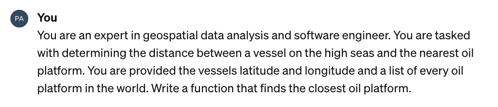
Let me provide an introductory example of a small piece of code generated by an LLM and the steps needed to make it useful. A common task in geospatial analysis is to measure the distance between a location on Earth and some other set of coordinates. Consider the following prompt.
Here is the immediate output:
import math

def haversine(lat1, lon1, lat2, lon2):
    # Radius of the Earth in kilometers
    R = 6371.0

    # Convert degrees to radians
    lat1_rad = math.radians(lat1)
    lon1_rad = math.radians(lon1)
    lat2_rad = math.radians(lat2)
    lon2_rad = math.radians(lon2)

    # Differences in coordinates
    dlat = lat2_rad - lat1_rad
    dlon = lon2_rad - lon1_rad

    # Haversine formula
    a = math.sin(dlat / 2)**2 + math.cos(lat1_rad) * math.cos(lat2_rad) * math.sin(dlon / 2)**2
    c = 2 * math.atan2(math.sqrt(a), math.sqrt(1 - a))

    # Distance in kilometers
    distance = R * c

    return distance

def find_closest_oil_platform(vessel_lat, vessel_lon, platforms):
    closest_platform = None
    min_distance = float('inf')

    for platform in platforms:
        distance = haversine(vessel_lat, vessel_lon, platform['latitude'], platform['longitude'])
        if distance < min_distance:
            min_distance = distance
            closest_platform = platform

    return closest_platform, min_distance
How good is that code?
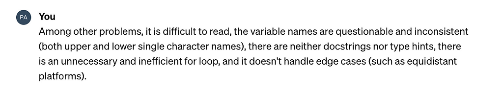
The quality of the code is quite poor. Among other issues, it is difficult to read due to questionable and inconsistent variable names, including both upper and lower single-character names. Additionally, it lacks docstrings and type hints, includes an unnecessary and inefficient for loop, and fails to handle edge cases, such as equidistant platforms.
Let’s simply say so:
from typing import Tuple, List
import numpy as np

def haversine_vectorized(vessel_lat: float, vessel_lon: float, platform_lats: np.ndarray, platform_lons: np.ndarray) -> np.ndarray:
    """
    Calculate the Haversine distance between a vessel and multiple platforms in a vectorized manner.

    Parameters:
    - vessel_lat: Latitude of the vessel in decimal degrees.
    - vessel_lon: Longitude of the vessel in decimal degrees.
    - platform_lats: Numpy array of latitudes of oil platforms in decimal degrees.
    - platform_lons: Numpy array of longitudes of oil platforms in decimal degrees.

    Returns:
    - distances: Numpy array of distances from the vessel to each platform in kilometers.
    """
    # Convert decimal degrees to radians
    lat1, lon1, lat2, lon2 = map(np.radians, [vessel_lat, vessel_lon, platform_lats, platform_lons])

    # Haversine formula
    dlat = lat2 - lat1
    dlon = lon2 - lon1
    a = np.sin(dlat/2)**2 + np.cos(lat1) * np.cos(lat2) * np.sin(dlon/2)**2
    c = 2 * np.arctan2(np.sqrt(a), np.sqrt(1-a))
    r = 6371  # Radius of Earth in kilometers
    return c * r

def find_closest_platform(vessel_lat: float, vessel_lon: float, platform_lats: np.ndarray, platform_lons: np.ndarray) -> Tuple[List[int], float]:
    """
    Finds the closest oil platform(s) to a vessel given arrays of platform latitudes and longitudes, handling equidistant platforms.

    Parameters:
    - vessel_lat: Latitude of the vessel in decimal degrees.
    - vessel_lon: Longitude of the vessel in decimal degrees.
    - platform_lats: Numpy array of latitudes for oil platforms.
    - platform_lons: Numpy array of longitudes for oil platforms.

    Returns:
    - A tuple containing a list of indices of the closest platforms and the distance to them in kilometers.
    """
    # Calculate distances to all platforms
    distances = haversine_vectorized(vessel_lat, vessel_lon, platform_lats, platform_lons)

    # Find the minimum distance
    min_distance = np.min(distances)

    # Find all indices with the minimum distance
    closest_indices = np.where(distances == min_distance)[0].tolist()

    # Return the indices of all closest platforms and the minimum distance
    return closest_indices, min_distance
The revised code is significantly improved. It is easier to read, includes docstrings and type hints, and the for-loop has been replaced with a much more efficient vector computation.
But how “good” it is, and more importantly, whether it satisfies the requirements depends on the context in which the code will be run. In doing so, remember that humans cannot effectively evaluate code quality outside of a much richer context than a few lines of code. And, unsurprisingly, neither can LLMs.
For example, is the accuracy of the implementation sufficient for the expected users? How often will the code run? Once a year? Once a microsecond? What hardware is available? Is the anticipated usage and scale such that it is worth looking for small optimizations? After factoring in your salary, is it worth doing so?
Let’s evaluate the code taking the above into account.
With respect to accuracy, the haversine formula is good but not great because it assumes the earth is a sphere, but the earth is an oblate spheroid. That distinction matters when millimeter precision is needed over massive distances. If it does, there are more accurate formulas (such as Vincenty’s formula), but those come with performance trade-offs. Because the users of this code would not benefit from millimeter precision (nor is that even relevant because the error in the satellite imagery-derived vessel coordinates is the limiting factor), the haversine function is a reasonable choice in terms of accuracy.
Is the code fast enough? There are only thousands of offshore oil platforms. Computing the distance to each one, especially with vector computations, is very efficient. If this code were used in other contexts, such as the distance to any point on shore (where there are billions of coastal points), a “divide and conquer” approach would be preferable. In production, I knew this function would run on the order of 100 million times per day on a VM that would be as small as possible to minimize compute costs.
Given all of that additional context, the above implementation is reasonable. Recall that means the code should then be tested (I avoid writing tests with LLMs) and peer-reviewed (by humans) before merging.
Part 2: Stepping On the Gas
Auto-generating useful functions like the above already saves time, but the value add compounds when you leverage LLMs to generate entire libraries with dependencies across modules, documentation, visualizations (via multimodal capabilities), READMEs, CLIs, and more.
Let’s create, train, evaluate, and infer a novel computer vision model from scratch with extensive aid from LLMs. As a motivating example, consider this recently published paper on “Keypoints Method for Recognition of Ship Wake Components in Sentinel-2 Images by Deep Learning” (Del Prete et al., IEEE GRSL, 2023).

Why should anyone care about the direction ships are traveling in satellite imagery and what makes this task non-trivial?
Determining a vessels course from static imagery is a valuable insight for organizations monitoring human activity in their waters. For example, knowing that a vessel is approaching a marine protected area might be cause for alarm or interception. The spatial resolution of global-scale publicly available satellite imagery is generally insufficient to adequately assess a vessel's orientation, especially for smaller vessels that occupy at most a few pixels (Sentinel-2 imagery is 10 meters/pixel). However, the wakes of even small vessels can be quite large, and that context allows one to determine the vessel's orientation and the direction it's traveling, even when it is impossible to identify the stern (back) of the boat.
The approach taken by the authors was compelling because the model described in the paper was built from EfficientNetB0, which is small enough to run cheaply at scale. I wasn’t able to find any relevant code, but the authors did make the dataset, including annotations, publicly available (kudos!).
Let’s get started!
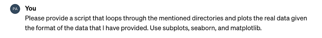
As is typical for any new ML project, it is informative to first visualize the data.
import os
import json
from PIL import Image, ImageDraw
import matplotlib.pyplot as plt
import seaborn as sns

# Define the path to your data directory
data_dir = "/path/to/your/data"  # Adjust this to the path of your data directory
annotations_dir = os.path.join(data_dir, "annotations")
images_dir = os.path.join(data_dir, "imgs")

# Initialize Seaborn for better visual aesthetics
sns.set(style="whitegrid", palette="muted")

# Create a list to hold file paths for images and their corresponding annotations
image_files = []
annotation_files = []

# Loop through the annotations directory to get the list of annotation files
for annotation_file in os.listdir(annotations_dir):
    if annotation_file.endswith(".json"):
        annotation_path = os.path.join(annotations_dir, annotation_file)
        image_file = annotation_file.replace(".json", ".png")  # Assuming image file names match annotation file names
        image_path = os.path.join(images_dir, image_file)

        # Check if the corresponding image file exists
        if os.path.exists(image_path):
            annotation_files.append(annotation_path)
            image_files.append(image_path)

# Plotting
num_examples = min(len(image_files), 10)  # Limiting to 10 examples for visualization
fig, axes = plt.subplots(2, 5, figsize=(20, 8))

for idx, (image_path, annotation_path) in enumerate(zip(image_files[:num_examples], annotation_files[:num_examples])):
    # Load the image
    img = Image.open(image_path).convert("RGB")  # Ensure the image is treated as RGB
    draw = ImageDraw.Draw(img)

    # Load the corresponding annotations and draw keypoints
    with open(annotation_path, 'r') as f:
        annotations = json.load(f)
        for point in annotations["tooltips"]:
            x, y = point["x"], point["y"]
            # Draw keypoints in cyan for visibility
            draw.ellipse([(x-10, y-10), (x+10, y+10)], fill='cyan', outline='black')

    # Plot the image with keypoints
    ax = axes[idx // 5, idx % 5]
    ax.imshow(img)
    ax.axis('off')
    ax.set_title(f"Image {idx+1}")

plt.tight_layout()
plt.show()
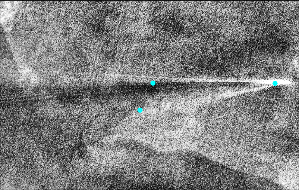
Which resulted in the following:
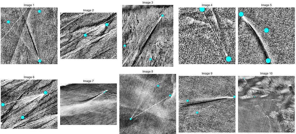
These plots indicate a few important points. First, the number of annotated keypoints (cyan dots) varies. Second, the images are grayscale and exhibit different shapes. Third, there is significant heterogeneity in this, albeit relatively small, sample. Keeping all of that in mind, let’s write the dataset loader, neural network definition, training, and validation loops. We will provide some context to our LLM before asking for the code.
Which resulted in the following output:
import os
import json
import torch
from torch.utils.data import Dataset, DataLoader
from torchvision import transforms
from torchvision.io import read_image
from typing import Tuple, List

class WakeDataset(Dataset):
    """
    Custom Dataset for loading wake detection imagery and annotations, with preprocessing for EfficientNet.
    Images are grayscale and will be converted to three-channel images for model compatibility.
    """

    def __init__(self, annotations_dir: str, images_dir: str, transform=None):
        """
        Initializes the dataset with paths to annotations and images directories, and a transform.

        Parameters:
        - annotations_dir: Path to the directory containing annotation JSON files.
        - images_dir: Path to the directory containing grayscale image files.
        - transform: A torchvision.transforms transform to be applied on a sample.
        """
        self.annotations_dir = annotations_dir
        self.images_dir = images_dir
        self.transform = transform if transform else self.default_transform()
        self.annotations = self._load_annotations()

    def default_transform(self):
        """
        Defines the default transform to resize images, convert them to three-channel format, and to tensors.

        Returns:
        - A torchvision.transforms composition for image preprocessing.
        """
        return transforms.Compose([
            transforms.Resize((224, 224)),  # Resize to the input size for EfficientNet
            transforms.Grayscale(num_output_channels=3),  # Convert grayscale to three-channel
            transforms.ConvertImageDtype(torch.float),  # Ensures image is a float tensor
        ])

    def _load_annotations(self) -> List[Tuple[str, List[int]]]:
        """
        Loads and filters annotations with at least 2 keypoints.

        Returns:
        - A list of tuples, where each tuple contains the image filename and its keypoints.
        """
        annotations = []
        for filename in os.listdir(self.annotations_dir):
            if not filename.endswith('.json'):
                continue
            filepath = os.path.join(self.annotations_dir, filename)
            with open(filepath, 'r') as f:
                data = json.load(f)
                if len(data['tooltips']) >= 2:  # Filter annotations with at least 2 keypoints
                    keypoints = [item for sublist in [[kp['x'], kp['y']] for kp in data['tooltips']] for item in sublist]
                    annotations.append((filename.replace('.json', '.png'), keypoints))
        return annotations

    def __len__(self) -> int:
        """
        Returns the number of items in the dataset.
        """
        return len(self.annotations)

    def __getitem__(self, idx) -> Tuple[torch.Tensor, torch.Tensor]:
        """
        Retrieves an item from the dataset at the specified index, with preprocessing for EfficientNet.

        Parameters:
        - idx: Index of the item to retrieve.

        Returns:
        - A tuple containing the preprocessed image tensor and its corresponding keypoints tensor.
        """
        img_name, keypoints = self.annotations[idx]
        img_path = os.path.join(self.images_dir, img_name)
        image = read_image(img_path)  # Load image
        keypoints = torch.tensor(keypoints + [0] * (6 - len(keypoints)), dtype=torch.float)  # Pad keypoints
        if self.transform:
            image = self.transform(image)
        return image, keypoints
The code looks reasonable, and it seems to have addressed some of the nuances of the problem. It’s not perfect (e.g., converting the images from grayscale to RGB in default_transform is a strange choice, and I prefer pathlib over os.listdir), but let's move on for now.
import torch
import torch.nn as nn
from torchvision import models
from typing import Tuple

class EfficientNetB0KeypointDetector(nn.Module):
    """
    A custom EfficientNet-B0 model for keypoint detection in grayscale images.
    The network modifies the input layer to accept single-channel images and
    adds a custom output layer for predicting a fixed number of keypoints.
    """

    def __init__(self, num_keypoints: int = 3):
        """
        Initializes the model.

        Parameters:
        - num_keypoints: The number of keypoints to predict. Default is 3,
                         corresponding to the maximum number of keypoints in the dataset.
        """
        super(EfficientNetB0KeypointDetector, self).__init__()
        self.num_keypoints = num_keypoints
        # Load a pre-trained EfficientNet-B0
        self.efficientnet_b0 = models.efficientnet_b0(pretrained=True)

        # Modify the first convolutional layer to accept single-channel (grayscale) images
        original_first_conv = self.efficientnet_b0.features[0][0]
        self.efficientnet_b0.features[0][0] = nn.Conv2d(
            in_channels=1,
            out_channels=original_first_conv.out_channels,
            kernel_size=original_first_conv.kernel_size,
            stride=original_first_conv.stride,
            padding=original_first_conv.padding,
            bias=False)

        # Modify the classifier to predict keypoints (num_keypoints * 2 because x, y for each keypoint)
        self.efficientnet_b0.classifier = nn.Linear(
            in_features=self.efficientnet_b0.classifier[1].in_features,
            out_features=num_keypoints * 2)

    def forward(self, x: torch.Tensor) -> torch.Tensor:
        """
        Forward pass of the network.

        Parameters:
        - x: Input tensor of shape (batch_size, 1, 224, 224)

        Returns:
        - A tensor of shape (batch_size, num_keypoints * 2) representing the predicted keypoints.
        """
        return self.efficientnet_b0(x)

# Example usage
if __name__ == "__main__":
    model = EfficientNetB0KeypointDetector()
    print(model)

    # Example input tensor (batch_size, channels, height, width)
    example_input = torch.randn(1, 1, 224, 224)
    output = model(example_input)
    print(output.shape)  # Expected shape: (1, 6) for 3 keypoints (each with x, y coordinates)
import os
import torch
import torch.nn as nn
import torch.optim as optim
from torch.utils.data import DataLoader
from dataset import WakeDataset, get_dataloader  # Assuming dataset.py is in the same directory
from net import EfficientNetB0KeypointDetector
from torchvision import transforms
import wandb

# Initialize Weights & Biases
wandb.init(project="wake_model_llm_assist", entity="your_wandb_entity", mode="offline")

def custom_collate_fn(batch):
    """
    Custom collate function to pad keypoints to a fixed size.

    Parameters:
    - batch: A list of tuples (image, keypoints).

    Returns:
    - Batched images and keypoints with padding as necessary.
    """
    images, keypoints = zip(*batch)
    images = torch.stack(images, 0)
    max_keypoints = 3 * 2  # Maximum number of keypoints (3) times 2 for (x, y)
    padded_keypoints = [torch.cat((kp, torch.zeros(max_keypoints - len(kp)))) for kp in keypoints]
    keypoints = torch.stack(padded_keypoints, 0)
    return images, keypoints

def train_one_epoch(model: nn.Module, dataloader: DataLoader, optimizer: optim.Optimizer, device: torch.device):
    """
    Trains the model for one epoch.

    Parameters:
    - model: The neural network model.
    - dataloader: DataLoader providing the training data.
    - optimizer: Optimizer used for model training.
    - device: The device to train on.
    """
    model.train()
    total_loss = 0.0
    for images, keypoints in dataloader:
        images, keypoints = images.to(device), keypoints.to(device)
        optimizer.zero_grad()
        outputs = model(images)
        loss = nn.MSELoss()(outputs, keypoints)
        loss.backward()
        optimizer.step()
        total_loss += loss.item()

    average_loss = total_loss / len(dataloader)
    wandb.log({"train_loss": average_loss})

def evaluate(model: nn.Module, dataloader: DataLoader, device: torch.device):
    """
    Evaluates the model on the validation set.

    Parameters:
    - model: The neural network model.
    - dataloader: DataLoader providing the validation data.
    - device: The device to evaluate on.
    """
    model.eval()
    total_loss = 0.0
    with torch.no_grad():
        for images, keypoints in dataloader:
            images, keypoints = images.to(device), keypoints.to(device)
            outputs = model(images)
            loss = nn.MSELoss()(outputs, keypoints)
            total_loss += loss.item()

    average_loss = total_loss / len(dataloader)
    wandb.log({"val_loss": average_loss})

def main():
    # Setup
    device = torch.device("cuda" if torch.cuda.is_available() else "cpu")
    model = EfficientNetB0KeypointDetector().to(device)
    optimizer = optim.Adam(model.parameters(), lr=1e-3)

    # DataLoaders
    train_dataloader = get_dataloader('path/to/train/annotations', 'path/to/train/images', batch_size=4, transform=transforms.ToTensor(), collate_fn=custom_collate_fn)
    val_dataloader = get_dataloader('path/to/val/annotations', 'path/to/val/images', batch_size=4, transform=transforms.ToTensor(), collate_fn=custom_collate_fn)

    # Training loop
    for epoch in range(num_epochs):
        train_one_epoch(model, train_dataloader, optimizer, device)
        evaluate(model, val_dataloader, device)
        # Log model checkpoints, images, or other metrics as needed
        wandb.log({})

if __name__ == "__main__":
    main()
I tried executing the code at this point but ran into multiple issues related to incorrect tensor shapes (recall the RGB/grayscale discrepancy and the custom collate function). I spent a few minutes debugging but ultimately just copied every module into the prompt window and asked for it to debug for me.
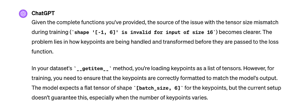
That was sufficient to resolve all of the lingering issues, and I kicked off training…which was absolutely glacial. I realized that I wasn’t using the Metal Performance Shaders (MPS) backend available on Apple silicon. I don’t generally train on my personal laptop, and MPS was new to me, but I added a conditional to use it.
Because the magnitude of the training data was modest (581 images), and given the fact that the EfficientNet was pre-trained on ImageNet — I chose to train for 1000 epochs.
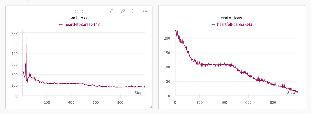
Note that there exist foundation models pre trained on satellite imagery (as opposed to ImageNet) which would (likely) be more performant for this task (see Bastani et. al.), but those nets are also much larger than EfficientNet, and therefore slower to train (and too new to be in LLM training corpora).
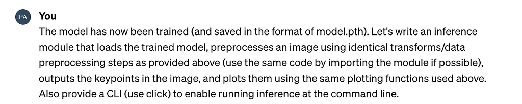
Let’s write an inference script, along with a CLI, to test the newly trained model.
import torch
from torchvision import transforms
from PIL import Image
import matplotlib.pyplot as plt
import click

# Assuming net.py contains the EfficientNetB0KeypointDetector class
# and dataset.py contains the transforms used during training
from net import EfficientNetB0KeypointDetector
from dataset import WakeDataset  # Modify as necessary to import transforms

def load_model(model_path):
    """Load the trained model from a file."""
    model = EfficientNetB0KeypointDetector()
    model.load_state_dict(torch.load(model_path))
    model.eval()  # Set the model to inference mode
    return model

def preprocess_image(image_path, transform):
    """Load and preprocess an image."""
    image = Image.open(image_path).convert("L")  # Assuming grayscale conversion as in your dataset
    image = transform(image)
    # Add batch dimension (BxCxHxW)
    image = image.unsqueeze(0)
    return image

def plot_keypoints(image, keypoints):
    """Plot keypoints on the image."""
    plt.imshow(image.squeeze(), cmap='gray')  # Remove batch dimension and show image
    plt.scatter(keypoints[:, 0], keypoints[:, 1], s=50, marker='.', c='red')
    plt.show()

@click.command()
@click.argument('model_path', type=click.Path(exists=True))
@click.argument('image_path', type=click.Path(exists=True))
def run_inference(model_path, image_path):
    """Run inference on an image using a trained model."""
    # Use the same transforms as during training
    transform = transforms.Compose([
        transforms.Resize((224, 224)),
        transforms.ToTensor(),
        transforms.Grayscale(num_output_channels=3),
    ])

    model = load_model(model_path)
    image = preprocess_image(image_path, transform)

    # Perform inference
    with torch.no_grad():
        keypoints = model(image)
        keypoints = keypoints.view(-1, 2).cpu().numpy()  # Reshape and convert to numpy for plotting

    # Load original image for plotting
    original_image = Image.open(image_path).convert("L")
    plot_keypoints(original_image, keypoints)

if __name__ == '__main__':
    run_inference()
Let’s try it!
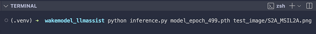
You can find the complete code with all of the modules, the model and weights (from the 500th epoch), and a readme on GitHub. I spent under an hour generating the entire library and far longer writing this article. Note that all of the above was completed on my personal laptop/development environment: MacBook Air M2 + VS Code + Copilot + autoformat on save (black, isort, etc) + a (.venv) Python 3.9.6.
Lessons Learned
- Provide the models with as much context as is relevant to solve the task. Remember that the model lacks many assumptions you may take for granted.
- LLM-generated code is typically far from perfect right off the bat, and it is difficult to predict how it will fail. For many reasons, it is helpful to have secondary assistance in your IDE (such as Copilot).
- When writing code with heavy dependence on LLMs, it is important to keep in mind that the limiting factor is waiting for the code to be written. Avoid asking for duplicated and redundant code that doesn’t require any changes. It is wasteful in terms of energy and it slows you down.
- LLMs have a difficult time ‘remembering’ every line of code that they have provided, and often it is worthwhile reminding them of the current state (especially when there are dependencies across multiple dependent modules).
- Be skeptical of LLM generated code. Validate as much as possible, using tests, visualizations, etc. And spend time where it matters. I spent far more time carefully evaluating the haversine function (where the performance mattered because of the anticipated scale) than I did the neural network (where the proof was more-so in the pudding). For the latter, I was most interested in failing fast.
Part 3: LLMs and the future of engineering
“There is nothing permanent except change” Heraclitus
With all of the hype surrounding LLMs and the massive amount of money exchanging hands, it is tempting to expect perfection at first blush. But effective use of these tools requires a willingness to experiment, learn, and adapt. Do LLMs change the fundamental structure of a software engineering team? Perhaps they will eventually, we have only seen the beginning of this new world. But we have already seen LLMs democratize access to code. Folks without programming experience can quickly and easily build functional prototypes. If your requirements are stringent, it may be prudent to leverage LLMs only in areas for which you already have expertise. My own experience is that LLMs dramatically reduce the time needed to arrive at performant code by a factor of ~10. If your personal experience is that they consistently output poor quality code, perhaps it is time to (re)evaluate the input.
Acknowledgments
Thanks to Ran Liu, Chris Hobson, and Bryce Blum for feedback.
Accelerating Engineering with LLMs was originally published in Towards Data Science on Medium, where people are continuing the conversation by highlighting and responding to this story.

Part 0: Skeptical Optimism
Part 1: Writing performant functions
Part 2: Stepping on the Gas
Part 3: LLMs and the future of engineering
Part 0: Skeptical Optimism
Steve Jobs famously likened the computer to a “bicycle for the mind.” However, the context in which he made that claim is less well-known. He was referring to the efficiency of locomotion for all different species on the planet.
“And the Condor won, came in at the top of the list, surpassed everything else, and humans came in about a third of the way down the list … But, a human riding a bicycle blew away the Condor, all the way off the top of the list. And it made a really big impression on me that we humans are tool builders, and that we can fashion tools that amplify these inherent abilities that we have to spectacular magnitudes. And so for me, a computer has always been a bicycle of the mind, something that takes us far beyond our inherent abilities and I think were just at the early stages of this tool, and already we have seen enormous changes and I think that’s nothing compared to what’s coming in the next 100 years” Steve Jobs (1990)
LLMs as tools to accelerate software development have been polarizing. Many people consider auto-generated code so poor that their use is net negative. At the other end of the spectrum, many headlines proclaim that programming is dead. There are already many research papers attempting objective evaluations of the performance of LLMs on benchmark code quality datasets such as HumanEval or MBPP. These evaluations are important for advancing the field but are not the objective of this article.
The goal here is to provide practical recommendations for developers, especially those reluctant to leverage these models. Fair warning: I believe that one’s efficiency can indeed soar to “spectacular magnitudes” with the appropriate use of this technology.
Note that leveraging an LLM doesn’t guarantee performant code. Even the latest and greatest models make egregious mistakes. But remember, the best human engineers make mistakes too. That is why we don’t ship code without safeguards, such as automated testing and peer review. LLMs haven’t changed the meaning of best practices, but they may have changed how easy it is to achieve them.
Does it even matter how fast you can write performant code?
I would be surprised if most professional software engineers spent the majority of their time physically tapping keys on the keyboard. If they did, we would probably take the idea of using “lines of code” as a performance metric more seriously. I suspect that engineers spend a much larger proportion of their time determining what code needs to be written in the first place. LLMs are not capable of such abstract reasoning (yet) — OpenAI and many others are working hard to codify those steps, but that will likely require paradigm shifts beyond simply scaling the parameters or training data. However, LLMs can already be used to massively accelerate a significant fraction of your work.
Part 1: Writing performant functions
Let me provide an introductory example of a small piece of code generated by an LLM and the steps needed to make it useful. A common task in geospatial analysis is to measure the distance between a location on Earth and some other set of coordinates. Consider the following prompt.
Here is the immediate output:
import math

def haversine(lat1, lon1, lat2, lon2):
    # Radius of the Earth in kilometers
    R = 6371.0

    # Convert degrees to radians
    lat1_rad = math.radians(lat1)
    lon1_rad = math.radians(lon1)
    lat2_rad = math.radians(lat2)
    lon2_rad = math.radians(lon2)

    # Differences in coordinates
    dlat = lat2_rad - lat1_rad
    dlon = lon2_rad - lon1_rad

    # Haversine formula
    a = math.sin(dlat / 2)**2 + math.cos(lat1_rad) * math.cos(lat2_rad) * math.sin(dlon / 2)**2
    c = 2 * math.atan2(math.sqrt(a), math.sqrt(1 - a))

    # Distance in kilometers
    distance = R * c

    return distance

def find_closest_oil_platform(vessel_lat, vessel_lon, platforms):
    closest_platform = None
    min_distance = float('inf')

    for platform in platforms:
        distance = haversine(vessel_lat, vessel_lon, platform['latitude'], platform['longitude'])
        if distance < min_distance:
            min_distance = distance
            closest_platform = platform

    return closest_platform, min_distance
How good is that code?
The quality of the code is quite poor. Among other issues, it is difficult to read due to questionable and inconsistent variable names, including both upper and lower single-character names. Additionally, it lacks docstrings and type hints, includes an unnecessary and inefficient for loop, and fails to handle edge cases, such as equidistant platforms.
Let’s simply say so:
from typing import Tuple, List
import numpy as np

def haversine_vectorized(vessel_lat: float, vessel_lon: float, platform_lats: np.ndarray, platform_lons: np.ndarray) -> np.ndarray:
    """
    Calculate the Haversine distance between a vessel and multiple platforms in a vectorized manner.

    Parameters:
    - vessel_lat: Latitude of the vessel in decimal degrees.
    - vessel_lon: Longitude of the vessel in decimal degrees.
    - platform_lats: Numpy array of latitudes of oil platforms in decimal degrees.
    - platform_lons: Numpy array of longitudes of oil platforms in decimal degrees.

    Returns:
    - distances: Numpy array of distances from the vessel to each platform in kilometers.
    """
    # Convert decimal degrees to radians
    lat1, lon1, lat2, lon2 = map(np.radians, [vessel_lat, vessel_lon, platform_lats, platform_lons])

    # Haversine formula
    dlat = lat2 - lat1
    dlon = lon2 - lon1
    a = np.sin(dlat/2)**2 + np.cos(lat1) * np.cos(lat2) * np.sin(dlon/2)**2
    c = 2 * np.arctan2(np.sqrt(a), np.sqrt(1-a))
    r = 6371  # Radius of Earth in kilometers
    return c * r

def find_closest_platform(vessel_lat: float, vessel_lon: float, platform_lats: np.ndarray, platform_lons: np.ndarray) -> Tuple[List[int], float]:
    """
    Finds the closest oil platform(s) to a vessel given arrays of platform latitudes and longitudes, handling equidistant platforms.

    Parameters:
    - vessel_lat: Latitude of the vessel in decimal degrees.
    - vessel_lon: Longitude of the vessel in decimal degrees.
    - platform_lats: Numpy array of latitudes for oil platforms.
    - platform_lons: Numpy array of longitudes for oil platforms.

    Returns:
    - A tuple containing a list of indices of the closest platforms and the distance to them in kilometers.
    """
    # Calculate distances to all platforms
    distances = haversine_vectorized(vessel_lat, vessel_lon, platform_lats, platform_lons)

    # Find the minimum distance
    min_distance = np.min(distances)

    # Find all indices with the minimum distance
    closest_indices = np.where(distances == min_distance)[0].tolist()

    # Return the indices of all closest platforms and the minimum distance
    return closest_indices, min_distance
The revised code is significantly improved. It is easier to read, includes docstrings and type hints, and the for-loop has been replaced with a much more efficient vector computation.
But how “good” it is, and more importantly, whether it satisfies the requirements depends on the context in which the code will be run. In doing so, remember that humans cannot effectively evaluate code quality outside of a much richer context than a few lines of code. And, unsurprisingly, neither can LLMs.
For example, is the accuracy of the implementation sufficient for the expected users? How often will the code run? Once a year? Once a microsecond? What hardware is available? Is the anticipated usage and scale such that it is worth looking for small optimizations? After factoring in your salary, is it worth doing so?
Let’s evaluate the code taking the above into account.
With respect to accuracy, the haversine formula is good but not great because it assumes the earth is a sphere, but the earth is an oblate spheroid. That distinction matters when millimeter precision is needed over massive distances. If it does, there are more accurate formulas (such as Vincenty’s formula), but those come with performance trade-offs. Because the users of this code would not benefit from millimeter precision (nor is that even relevant because the error in the satellite imagery-derived vessel coordinates is the limiting factor), the haversine function is a reasonable choice in terms of accuracy.
Is the code fast enough? There are only thousands of offshore oil platforms. Computing the distance to each one, especially with vector computations, is very efficient. If this code were used in other contexts, such as the distance to any point on shore (where there are billions of coastal points), a “divide and conquer” approach would be preferable. In production, I knew this function would run on the order of 100 million times per day on a VM that would be as small as possible to minimize compute costs.
Given all of that additional context, the above implementation is reasonable. Recall that means the code should then be tested (I avoid writing tests with LLMs) and peer-reviewed (by humans) before merging.
Part 2: Stepping On the Gas
Auto-generating useful functions like the above already saves time, but the value add compounds when you leverage LLMs to generate entire libraries with dependencies across modules, documentation, visualizations (via multimodal capabilities), READMEs, CLIs, and more.
Let’s create, train, evaluate, and infer a novel computer vision model from scratch with extensive aid from LLMs. As a motivating example, consider this recently published paper on “Keypoints Method for Recognition of Ship Wake Components in Sentinel-2 Images by Deep Learning” (Del Prete et al., IEEE GRSL, 2023).
Why should anyone care about the direction ships are traveling in satellite imagery and what makes this task non-trivial?
Determining a vessels course from static imagery is a valuable insight for organizations monitoring human activity in their waters. For example, knowing that a vessel is approaching a marine protected area might be cause for alarm or interception. The spatial resolution of global-scale publicly available satellite imagery is generally insufficient to adequately assess a vessel's orientation, especially for smaller vessels that occupy at most a few pixels (Sentinel-2 imagery is 10 meters/pixel). However, the wakes of even small vessels can be quite large, and that context allows one to determine the vessel's orientation and the direction it's traveling, even when it is impossible to identify the stern (back) of the boat.
The approach taken by the authors was compelling because the model described in the paper was built from EfficientNetB0, which is small enough to run cheaply at scale. I wasn’t able to find any relevant code, but the authors did make the dataset, including annotations, publicly available (kudos!).
Let’s get started!
As is typical for any new ML project, it is informative to first visualize the data.
import os
import json
from PIL import Image, ImageDraw
import matplotlib.pyplot as plt
import seaborn as sns

# Define the path to your data directory
data_dir = "/path/to/your/data"  # Adjust this to the path of your data directory
annotations_dir = os.path.join(data_dir, "annotations")
images_dir = os.path.join(data_dir, "imgs")

# Initialize Seaborn for better visual aesthetics
sns.set(style="whitegrid", palette="muted")

# Create a list to hold file paths for images and their corresponding annotations
image_files = []
annotation_files = []

# Loop through the annotations directory to get the list of annotation files
for annotation_file in os.listdir(annotations_dir):
    if annotation_file.endswith(".json"):
        annotation_path = os.path.join(annotations_dir, annotation_file)
        image_file = annotation_file.replace(".json", ".png")  # Assuming image file names match annotation file names
        image_path = os.path.join(images_dir, image_file)

        # Check if the corresponding image file exists
        if os.path.exists(image_path):
            annotation_files.append(annotation_path)
            image_files.append(image_path)

# Plotting
num_examples = min(len(image_files), 10)  # Limiting to 10 examples for visualization
fig, axes = plt.subplots(2, 5, figsize=(20, 8))

for idx, (image_path, annotation_path) in enumerate(zip(image_files[:num_examples], annotation_files[:num_examples])):
    # Load the image
    img = Image.open(image_path).convert("RGB")  # Ensure the image is treated as RGB
    draw = ImageDraw.Draw(img)

    # Load the corresponding annotations and draw keypoints
    with open(annotation_path, 'r') as f:
        annotations = json.load(f)
        for point in annotations["tooltips"]:
            x, y = point["x"], point["y"]
            # Draw keypoints in cyan for visibility
            draw.ellipse([(x-10, y-10), (x+10, y+10)], fill='cyan', outline='black')

    # Plot the image with keypoints
    ax = axes[idx // 5, idx % 5]
    ax.imshow(img)
    ax.axis('off')
    ax.set_title(f"Image {idx+1}")

plt.tight_layout()
plt.show()
Which resulted in the following:
These plots indicate a few important points. First, the number of annotated keypoints (cyan dots) varies. Second, the images are grayscale and exhibit different shapes. Third, there is significant heterogeneity in this, albeit relatively small, sample. Keeping all of that in mind, let’s write the dataset loader, neural network definition, training, and validation loops. We will provide some context to our LLM before asking for the code.
Which resulted in the following output:
import os
import json
import torch
from torch.utils.data import Dataset, DataLoader
from torchvision import transforms
from torchvision.io import read_image
from typing import Tuple, List

class WakeDataset(Dataset):
    """
    Custom Dataset for loading wake detection imagery and annotations, with preprocessing for EfficientNet.
    Images are grayscale and will be converted to three-channel images for model compatibility.
    """

    def __init__(self, annotations_dir: str, images_dir: str, transform=None):
        """
        Initializes the dataset with paths to annotations and images directories, and a transform.

        Parameters:
        - annotations_dir: Path to the directory containing annotation JSON files.
        - images_dir: Path to the directory containing grayscale image files.
        - transform: A torchvision.transforms transform to be applied on a sample.
        """
        self.annotations_dir = annotations_dir
        self.images_dir = images_dir
        self.transform = transform if transform else self.default_transform()
        self.annotations = self._load_annotations()

    def default_transform(self):
        """
        Defines the default transform to resize images, convert them to three-channel format, and to tensors.

        Returns:
        - A torchvision.transforms composition for image preprocessing.
        """
        return transforms.Compose([
            transforms.Resize((224, 224)),  # Resize to the input size for EfficientNet
            transforms.Grayscale(num_output_channels=3),  # Convert grayscale to three-channel
            transforms.ConvertImageDtype(torch.float),  # Ensures image is a float tensor
        ])

    def _load_annotations(self) -> List[Tuple[str, List[int]]]:
        """
        Loads and filters annotations with at least 2 keypoints.

        Returns:
        - A list of tuples, where each tuple contains the image filename and its keypoints.
        """
        annotations = []
        for filename in os.listdir(self.annotations_dir):
            if not filename.endswith('.json'):
                continue
            filepath = os.path.join(self.annotations_dir, filename)
            with open(filepath, 'r') as f:
                data = json.load(f)
                if len(data['tooltips']) >= 2:  # Filter annotations with at least 2 keypoints
                    keypoints = [item for sublist in [[kp['x'], kp['y']] for kp in data['tooltips']] for item in sublist]
                    annotations.append((filename.replace('.json', '.png'), keypoints))
        return annotations

    def __len__(self) -> int:
        """
        Returns the number of items in the dataset.
        """
        return len(self.annotations)

    def __getitem__(self, idx) -> Tuple[torch.Tensor, torch.Tensor]:
        """
        Retrieves an item from the dataset at the specified index, with preprocessing for EfficientNet.

        Parameters:
        - idx: Index of the item to retrieve.

        Returns:
        - A tuple containing the preprocessed image tensor and its corresponding keypoints tensor.
        """
        img_name, keypoints = self.annotations[idx]
        img_path = os.path.join(self.images_dir, img_name)
        image = read_image(img_path)  # Load image
        keypoints = torch.tensor(keypoints + [0] * (6 - len(keypoints)), dtype=torch.float)  # Pad keypoints
        if self.transform:
            image = self.transform(image)
        return image, keypoints
The code looks reasonable, and it seems to have addressed some of the nuances of the problem. It’s not perfect (e.g., converting the images from grayscale to RGB in default_transform is a strange choice, and I prefer pathlib over os.listdir), but let's move on for now.
import torch
import torch.nn as nn
from torchvision import models
from typing import Tuple

class EfficientNetB0KeypointDetector(nn.Module):
    """
    A custom EfficientNet-B0 model for keypoint detection in grayscale images.
    The network modifies the input layer to accept single-channel images and
    adds a custom output layer for predicting a fixed number of keypoints.
    """

    def __init__(self, num_keypoints: int = 3):
        """
        Initializes the model.

        Parameters:
        - num_keypoints: The number of keypoints to predict. Default is 3,
                         corresponding to the maximum number of keypoints in the dataset.
        """
        super(EfficientNetB0KeypointDetector, self).__init__()
        self.num_keypoints = num_keypoints
        # Load a pre-trained EfficientNet-B0
        self.efficientnet_b0 = models.efficientnet_b0(pretrained=True)

        # Modify the first convolutional layer to accept single-channel (grayscale) images
        original_first_conv = self.efficientnet_b0.features[0][0]
        self.efficientnet_b0.features[0][0] = nn.Conv2d(
            in_channels=1,
            out_channels=original_first_conv.out_channels,
            kernel_size=original_first_conv.kernel_size,
            stride=original_first_conv.stride,
            padding=original_first_conv.padding,
            bias=False)

        # Modify the classifier to predict keypoints (num_keypoints * 2 because x, y for each keypoint)
        self.efficientnet_b0.classifier = nn.Linear(
            in_features=self.efficientnet_b0.classifier[1].in_features,
            out_features=num_keypoints * 2)

    def forward(self, x: torch.Tensor) -> torch.Tensor:
        """
        Forward pass of the network.

        Parameters:
        - x: Input tensor of shape (batch_size, 1, 224, 224)

        Returns:
        - A tensor of shape (batch_size, num_keypoints * 2) representing the predicted keypoints.
        """
        return self.efficientnet_b0(x)

# Example usage
if __name__ == "__main__":
    model = EfficientNetB0KeypointDetector()
    print(model)

    # Example input tensor (batch_size, channels, height, width)
    example_input = torch.randn(1, 1, 224, 224)
    output = model(example_input)
    print(output.shape)  # Expected shape: (1, 6) for 3 keypoints (each with x, y coordinates)
import os
import torch
import torch.nn as nn
import torch.optim as optim
from torch.utils.data import DataLoader
from dataset import WakeDataset, get_dataloader  # Assuming dataset.py is in the same directory
from net import EfficientNetB0KeypointDetector
from torchvision import transforms
import wandb

# Initialize Weights & Biases
wandb.init(project="wake_model_llm_assist", entity="your_wandb_entity", mode="offline")

def custom_collate_fn(batch):
    """
    Custom collate function to pad keypoints to a fixed size.

    Parameters:
    - batch: A list of tuples (image, keypoints).

    Returns:
    - Batched images and keypoints with padding as necessary.
    """
    images, keypoints = zip(*batch)
    images = torch.stack(images, 0)
    max_keypoints = 3 * 2  # Maximum number of keypoints (3) times 2 for (x, y)
    padded_keypoints = [torch.cat((kp, torch.zeros(max_keypoints - len(kp)))) for kp in keypoints]
    keypoints = torch.stack(padded_keypoints, 0)
    return images, keypoints

def train_one_epoch(model: nn.Module, dataloader: DataLoader, optimizer: optim.Optimizer, device: torch.device):
    """
    Trains the model for one epoch.

    Parameters:
    - model: The neural network model.
    - dataloader: DataLoader providing the training data.
    - optimizer: Optimizer used for model training.
    - device: The device to train on.
    """
    model.train()
    total_loss = 0.0
    for images, keypoints in dataloader:
        images, keypoints = images.to(device), keypoints.to(device)
        optimizer.zero_grad()
        outputs = model(images)
        loss = nn.MSELoss()(outputs, keypoints)
        loss.backward()
        optimizer.step()
        total_loss += loss.item()

    average_loss = total_loss / len(dataloader)
    wandb.log({"train_loss": average_loss})

def evaluate(model: nn.Module, dataloader: DataLoader, device: torch.device):
    """
    Evaluates the model on the validation set.

    Parameters:
    - model: The neural network model.
    - dataloader: DataLoader providing the validation data.
    - device: The device to evaluate on.
    """
    model.eval()
    total_loss = 0.0
    with torch.no_grad():
        for images, keypoints in dataloader:
            images, keypoints = images.to(device), keypoints.to(device)
            outputs = model(images)
            loss = nn.MSELoss()(outputs, keypoints)
            total_loss += loss.item()

    average_loss = total_loss / len(dataloader)
    wandb.log({"val_loss": average_loss})

def main():
    # Setup
    device = torch.device("cuda" if torch.cuda.is_available() else "cpu")
    model = EfficientNetB0KeypointDetector().to(device)
    optimizer = optim.Adam(model.parameters(), lr=1e-3)

    # DataLoaders
    train_dataloader = get_dataloader('path/to/train/annotations', 'path/to/train/images', batch_size=4, transform=transforms.ToTensor(), collate_fn=custom_collate_fn)
    val_dataloader = get_dataloader('path/to/val/annotations', 'path/to/val/images', batch_size=4, transform=transforms.ToTensor(), collate_fn=custom_collate_fn)

    # Training loop
    for epoch in range(num_epochs):
        train_one_epoch(model, train_dataloader, optimizer, device)
        evaluate(model, val_dataloader, device)
        # Log model checkpoints, images, or other metrics as needed
        wandb.log({})

if __name__ == "__main__":
    main()
I tried executing the code at this point but ran into multiple issues related to incorrect tensor shapes (recall the RGB/grayscale discrepancy and the custom collate function). I spent a few minutes debugging but ultimately just copied every module into the prompt window and asked for it to debug for me.
That was sufficient to resolve all of the lingering issues, and I kicked off training…which was absolutely glacial. I realized that I wasn’t using the Metal Performance Shaders (MPS) backend available on Apple silicon. I don’t generally train on my personal laptop, and MPS was new to me, but I added a conditional to use it.
Because the magnitude of the training data was modest (581 images), and given the fact that the EfficientNet was pre-trained on ImageNet — I chose to train for 1000 epochs.
Note that there exist foundation models pre trained on satellite imagery (as opposed to ImageNet) which would (likely) be more performant for this task (see Bastani et. al.), but those nets are also much larger than EfficientNet, and therefore slower to train (and too new to be in LLM training corpora).
Let’s write an inference script, along with a CLI, to test the newly trained model.
import torch
from torchvision import transforms
from PIL import Image
import matplotlib.pyplot as plt
import click

# Assuming net.py contains the EfficientNetB0KeypointDetector class
# and dataset.py contains the transforms used during training
from net import EfficientNetB0KeypointDetector
from dataset import WakeDataset  # Modify as necessary to import transforms

def load_model(model_path):
    """Load the trained model from a file."""
    model = EfficientNetB0KeypointDetector()
    model.load_state_dict(torch.load(model_path))
    model.eval()  # Set the model to inference mode
    return model

def preprocess_image(image_path, transform):
    """Load and preprocess an image."""
    image = Image.open(image_path).convert("L")  # Assuming grayscale conversion as in your dataset
    image = transform(image)
    # Add batch dimension (BxCxHxW)
    image = image.unsqueeze(0)
    return image

def plot_keypoints(image, keypoints):
    """Plot keypoints on the image."""
    plt.imshow(image.squeeze(), cmap='gray')  # Remove batch dimension and show image
    plt.scatter(keypoints[:, 0], keypoints[:, 1], s=50, marker='.', c='red')
    plt.show()

@click.command()
@click.argument('model_path', type=click.Path(exists=True))
@click.argument('image_path', type=click.Path(exists=True))
def run_inference(model_path, image_path):
    """Run inference on an image using a trained model."""
    # Use the same transforms as during training
    transform = transforms.Compose([
        transforms.Resize((224, 224)),
        transforms.ToTensor(),
        transforms.Grayscale(num_output_channels=3),
    ])

    model = load_model(model_path)
    image = preprocess_image(image_path, transform)

    # Perform inference
    with torch.no_grad():
        keypoints = model(image)
        keypoints = keypoints.view(-1, 2).cpu().numpy()  # Reshape and convert to numpy for plotting

    # Load original image for plotting
    original_image = Image.open(image_path).convert("L")
    plot_keypoints(original_image, keypoints)

if __name__ == '__main__':
    run_inference()
Let’s try it!
You can find the complete code with all of the modules, the model and weights (from the 500th epoch), and a readme on GitHub. I spent under an hour generating the entire library and far longer writing this article. Note that all of the above was completed on my personal laptop/development environment: MacBook Air M2 + VS Code + Copilot + autoformat on save (black, isort, etc) + a (.venv) Python 3.9.6.
Lessons Learned
- Provide the models with as much context as is relevant to solve the task. Remember that the model lacks many assumptions you may take for granted.
- LLM-generated code is typically far from perfect right off the bat, and it is difficult to predict how it will fail. For many reasons, it is helpful to have secondary assistance in your IDE (such as Copilot).
- When writing code with heavy dependence on LLMs, it is important to keep in mind that the limiting factor is waiting for the code to be written. Avoid asking for duplicated and redundant code that doesn’t require any changes. It is wasteful in terms of energy and it slows you down.
- LLMs have a difficult time ‘remembering’ every line of code that they have provided, and often it is worthwhile reminding them of the current state (especially when there are dependencies across multiple dependent modules).
- Be skeptical of LLM generated code. Validate as much as possible, using tests, visualizations, etc. And spend time where it matters. I spent far more time carefully evaluating the haversine function (where the performance mattered because of the anticipated scale) than I did the neural network (where the proof was more-so in the pudding). For the latter, I was most interested in failing fast.
Part 3: LLMs and the future of engineering
“There is nothing permanent except change” Heraclitus
With all of the hype surrounding LLMs and the massive amount of money exchanging hands, it is tempting to expect perfection at first blush. But effective use of these tools requires a willingness to experiment, learn, and adapt. Do LLMs change the fundamental structure of a software engineering team? Perhaps they will eventually, we have only seen the beginning of this new world. But we have already seen LLMs democratize access to code. Folks without programming experience can quickly and easily build functional prototypes. If your requirements are stringent, it may be prudent to leverage LLMs only in areas for which you already have expertise. My own experience is that LLMs dramatically reduce the time needed to arrive at performant code by a factor of ~10. If your personal experience is that they consistently output poor quality code, perhaps it is time to (re)evaluate the input.
Acknowledgments
Thanks to Ran Liu, Chris Hobson, and Bryce Blum for feedback.
Accelerating Engineering with LLMs was originally published in Towards Data Science on Medium, where people are continuing the conversation by highlighting and responding to this story.
Denial of responsibility! Techno Blender is an automatic aggregator of the all world’s media. In each content, the hyperlink to the primary source is specified. All trademarks belong to their rightful owners, all materials to their authors. If you are the owner of the content and do not want us to publish your materials, please contact us by email – [email protected]. The content will be deleted within 24 hours.