
Active Learning for Cell Imaging. Prioritize labeling of cell imaging… | by Nimrod Berman | Jul, 2022
Prioritize labeling of cell imaging samples based on the prospective impact of their label on the model’s performance.
Adi Nissim, Noam Siegel, Nimrod Berman
One of the main obstacles standing in front of many machine learning tasks is the lack of labeled data. Labeling data might be exhausting and expensive. Thus, many times it is not reasonable to even try to solve a problem using machine learning methods due to lack of labels.
To alleviate this problem, a field in machine learning has emerged, called Active Learning. Active Learning is a method in machine learning that provides a framework for prioritizing the unlabeled data samples based on the labeled data that a model already saw. We won’t get into detail about it, you can read Active Learning in Machine Learning article that deeply explains the basics of it.
Data science in cell imaging is a research field that rapidly advances. Yet, as in other machine learinng domains, labels are expensive. To accomodate this problem, we show in this article an end to end work on image cell active-learning classification task of red and white blood cells.
Our goal is to introduce the combination of Biology and Active Learning and help others to solve similar and more complicated tasks in the Biology domain using Active Learning methods.
The article is consructed of 3 main parts:
- Cell Image Preprocessing — where we show how to preprocess unsegmented blood cells images.
- Cell Feature Extraction Using Cell Profiler — where we show how to extract morphological feature from biological cell photo-images to use as features for machine learning models.
- Using Active Learning — where we show an experiment that simulates the use of active learning along with a comparison to not using active learning.
The data set
We will use a dataset of blood cell images which was uploaded to GitHub as well as Kaggle under the MIT license. Each image is labeled according to Red-Blood-Cell (RBC) vs White-Blood-Cell (WBC) classes. There are additional labels for the 4 kinds of WBCs (Eosinophil, Lymphocyte, Monocyte, and Neutrophil) but we did not use these labels in our study.
Here is an example of a full-sized, raw image from the dataset:
Creating a Samples DataFrame
We found that the original dataset contains an export.py script which parses the XML annotations into a CSV table with the filenames, cell type labels and bounding boxes for each cell.
Unfortunately, the original script did not include a cell_id column which is necessary because we are classifying individual cells. So, we slightly modified the code to include this column, as well as choose new filenames which include the image_id and cell_id:
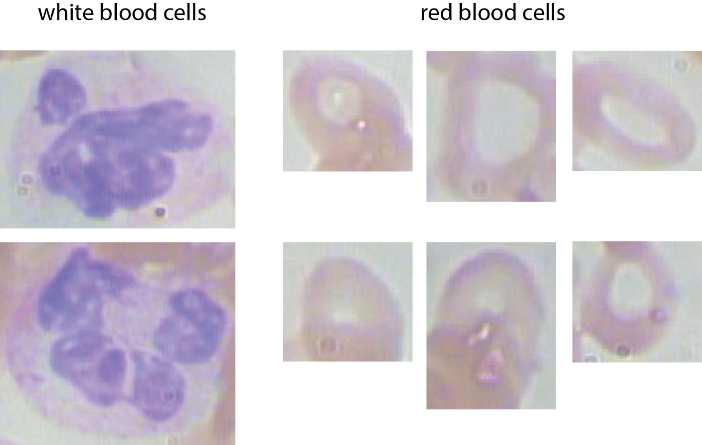
The first step in order to be able to work with the data, is to crop the full-sized images based on the bounding-box coordinates. This results in funky cell-images:
And, here is the code:
For your convenience, we forked the original repository and uploaded the cropped images to GitHub! They can be found at:
https://github.com/noamsgl/BCCD_Dataset/tree/master/BCCD/cropped
That’s it with the preprocessing! Now, go ahead and extract features with CellProfiler.
CellProfiler is a free open-sorce image analysis software, designed to automate quantitative measurement phenotyps from large-scale cell images. CellProfiler has a user-friendly graphical-user-interface (GUI), allowing you to use built-in piplines as well as building your own tailored to your specific needs, using a variety of measurements and features.
Getting started:
First, download Cellprofiler. If CellProfiler will not open, you may need to install the Visual C++ Redistributable.
Once the GUI pops up, load images and write organized metadata into CellProfiler. If you choose to build your own pipeline, here you may find the list of modules available through CellProfiler. Most of the modules are divided into three main groups: Image processing, Object processing and Measurements. You can save your pipeline configuration and reuse it or share it with the world.
Now we will demonstrate the feature extraction process:
- Image processing – You can perform several manipulations on the images before activating the features. For example, converting the image from color to grayscale:

- Object processing – These modules detect and identify, or allow you to manipulate objects in the image.

- Measurements – Now, after we have activated image processing modules, and we have identified primary objects in it, measurements known to be helpful for cell profiling can be calculated per object and summarized per image.

With CellProfiler you can save the output data to spreedsheets or other types of databases. We saved our output as a .CSV file and loaded it to Python as features for the machine learning model.
OK, so now finally we have tabular data that we can try to experiment with. We want to experiment whether using an Active Learning strategy can save time by labeling less data and getting higher accuracies. Our hypothesis is that using active learning, we could potentially save precious time and effort, by reducing significantly the amount of labeled data required to train a machine learning model on a cell classification task.
Active Learning Framework
Before we dive into our experiment, we want to conduct a quick introduction to modAL. ModAL is an active learning framework for python. It shares the sklearn API so it is really easy to integrate it into your code if you are working with Sklearn. This framework allows you to easily use different state of the art Active Learning strategies. Their documentation is easy to follow and we really recommend using it in your Active Learning pipeline.
Active Learning VS Random appoach
The Experiment
To validate our hypothesis we will conduct an experiment that will compare a Random Subsampling strategy to add new labeled data, to an Active Learning strategy. We will start training 2 Logistic Regressions estimators with a few same labeled samples. Then, we are going to use the Random strategy for one model and the Active Learning strategy for the second model. We will explain later how this is going to work exactly.
Preparing the Data for the Experiment
We first load the features created by the Cell Profiler. To make things easier, we filter platelets which are colorless blood cells. We keep only red and white blood cells. Thus we are trying to solve a binary classification problem – RBC vs WBC. Then we set the label using sklearn label encoder, extract the learning features from the data to X and finally split the data to train and test.
Preparing the data for the experiment
Now we will set the models
The Dummy learner will be the model that will use the Random strategy while the active learner will be using an Active Learning strategy. To instantiate an active learner model, we use ActiveLearner object from modAL package. In the ‘estimator’ field, you can insert any sklearn model that will be fit to the data. The ‘query_strategy’ field is where you choose a specific Active Learning strategy. We used ‘uncertainty_sampling()’. For more information check out modAL documentation.
Spliting the training data
To create our virtual strategies experiment, we split the training data into 2 groups. The first one is training data that we know its labels and we will use it to train our models. The second one is training data that we act like we don’t know its labels. We set the known train size to 5 samples.
Simulate Active VS Dummy
Now, we will run 298 epochs where in each one we will train each model, choose the next sample that we will insert the ‘base’ data by the strategy of each model, and measure its accuray along each epoch. We will use average precision score to measure the preformance of the models. We chose this metric because of the imbalanced nature of the dataset.
To pick the next sample in the Random strategy, we will just add the next sample in the ‘new’ group of the dummy dataset. This dataset is shuffled so no need for reshuffling. To pick the next sample with the active learning framework, we will use the ActiveLearner method called ‘query’ which gets the unlabeled data of the ‘new’ group and returns the index of the sample that he recommends to add to the training ‘base’ group. Each sample that we pick will remove from the ‘new’ group so that no sample can be choosen twice or more.
In this example we added 1 sample in each iteration. In the real world, it might be more practical to sample a batch of k samples at a time.
Results
The differences between the strategies are striking!
We can see that using active learning we are able to reach average precision 0.9 score with only 25 samples! While with the dummy strategy requires 175 samples to reach the same accuracy! What a gap!
In addition, the Active model reaches high score of almost 0.99 while the dummy stops around 0.95! If we would use all the data then they will reach the same score eventually, but for our purpose we limited to 300 random samples from the dataset.
Code for the plot:
Supervised machine learning techniques to cell image classification require labeled data sets. The success of these techniques will be constrained by out-of-budget labels as data grows. To overcome this challenge, we show how to easily use Active Learning to select the fewest number of images to label and still achieve the highest classification scores. Our experiments show that the Active Learning strategy scores 0.9 average precision (a metric suitable for imbalanced datasets) with just 25 labels, compared to 0.4 with a random selection dummy strategy.
Cell imaging has made a large contribution to the fields of biology, medicine and pharmacology. It is used to identify the type of the cell, its toxicity, integrity and phase, and that information is essential for healthcare providers and scientists to identify disease and expand our understanding of cell biology.
Previously, analyzing cell images required valuable professional human capital. Modern improvement in the quality and availability of microscopy methods as well as advanced machine learning algorithms, have enabled the data science field to revolutionize cell imaging. These new technologies have led to dynamic and multidimensional quality databases, and the ability to process this modern cell imaging data is having a crucial role in the advancement of the cell biology field.
Hopefully, cell biologists and others will find this article helpful to understand active learning strategies, how to implement them in custom machine learning solutions, and find it easier to use data science methods in their research.
Finally, you are welcome to share your thoughts and suggestions in the comments section after using Active Learning for your projects!
[1] Active Learning in Machine Learning | by Ana Solaguren-Beascoa, PhD | Towards Data Science
Prioritize labeling of cell imaging samples based on the prospective impact of their label on the model’s performance.
Adi Nissim, Noam Siegel, Nimrod Berman
One of the main obstacles standing in front of many machine learning tasks is the lack of labeled data. Labeling data might be exhausting and expensive. Thus, many times it is not reasonable to even try to solve a problem using machine learning methods due to lack of labels.
To alleviate this problem, a field in machine learning has emerged, called Active Learning. Active Learning is a method in machine learning that provides a framework for prioritizing the unlabeled data samples based on the labeled data that a model already saw. We won’t get into detail about it, you can read Active Learning in Machine Learning article that deeply explains the basics of it.
Data science in cell imaging is a research field that rapidly advances. Yet, as in other machine learinng domains, labels are expensive. To accomodate this problem, we show in this article an end to end work on image cell active-learning classification task of red and white blood cells.
Our goal is to introduce the combination of Biology and Active Learning and help others to solve similar and more complicated tasks in the Biology domain using Active Learning methods.
The article is consructed of 3 main parts:
- Cell Image Preprocessing — where we show how to preprocess unsegmented blood cells images.
- Cell Feature Extraction Using Cell Profiler — where we show how to extract morphological feature from biological cell photo-images to use as features for machine learning models.
- Using Active Learning — where we show an experiment that simulates the use of active learning along with a comparison to not using active learning.
The data set
We will use a dataset of blood cell images which was uploaded to GitHub as well as Kaggle under the MIT license. Each image is labeled according to Red-Blood-Cell (RBC) vs White-Blood-Cell (WBC) classes. There are additional labels for the 4 kinds of WBCs (Eosinophil, Lymphocyte, Monocyte, and Neutrophil) but we did not use these labels in our study.
Here is an example of a full-sized, raw image from the dataset:
Creating a Samples DataFrame
We found that the original dataset contains an export.py script which parses the XML annotations into a CSV table with the filenames, cell type labels and bounding boxes for each cell.
Unfortunately, the original script did not include a cell_id column which is necessary because we are classifying individual cells. So, we slightly modified the code to include this column, as well as choose new filenames which include the image_id and cell_id:
The first step in order to be able to work with the data, is to crop the full-sized images based on the bounding-box coordinates. This results in funky cell-images:
And, here is the code:
For your convenience, we forked the original repository and uploaded the cropped images to GitHub! They can be found at:
https://github.com/noamsgl/BCCD_Dataset/tree/master/BCCD/cropped
That’s it with the preprocessing! Now, go ahead and extract features with CellProfiler.
CellProfiler is a free open-sorce image analysis software, designed to automate quantitative measurement phenotyps from large-scale cell images. CellProfiler has a user-friendly graphical-user-interface (GUI), allowing you to use built-in piplines as well as building your own tailored to your specific needs, using a variety of measurements and features.
Getting started:
First, download Cellprofiler. If CellProfiler will not open, you may need to install the Visual C++ Redistributable.
Once the GUI pops up, load images and write organized metadata into CellProfiler. If you choose to build your own pipeline, here you may find the list of modules available through CellProfiler. Most of the modules are divided into three main groups: Image processing, Object processing and Measurements. You can save your pipeline configuration and reuse it or share it with the world.
Now we will demonstrate the feature extraction process:
- Image processing – You can perform several manipulations on the images before activating the features. For example, converting the image from color to grayscale:
- Object processing – These modules detect and identify, or allow you to manipulate objects in the image.
- Measurements – Now, after we have activated image processing modules, and we have identified primary objects in it, measurements known to be helpful for cell profiling can be calculated per object and summarized per image.
With CellProfiler you can save the output data to spreedsheets or other types of databases. We saved our output as a .CSV file and loaded it to Python as features for the machine learning model.
OK, so now finally we have tabular data that we can try to experiment with. We want to experiment whether using an Active Learning strategy can save time by labeling less data and getting higher accuracies. Our hypothesis is that using active learning, we could potentially save precious time and effort, by reducing significantly the amount of labeled data required to train a machine learning model on a cell classification task.
Active Learning Framework
Before we dive into our experiment, we want to conduct a quick introduction to modAL. ModAL is an active learning framework for python. It shares the sklearn API so it is really easy to integrate it into your code if you are working with Sklearn. This framework allows you to easily use different state of the art Active Learning strategies. Their documentation is easy to follow and we really recommend using it in your Active Learning pipeline.
Active Learning VS Random appoach
The Experiment
To validate our hypothesis we will conduct an experiment that will compare a Random Subsampling strategy to add new labeled data, to an Active Learning strategy. We will start training 2 Logistic Regressions estimators with a few same labeled samples. Then, we are going to use the Random strategy for one model and the Active Learning strategy for the second model. We will explain later how this is going to work exactly.
Preparing the Data for the Experiment
We first load the features created by the Cell Profiler. To make things easier, we filter platelets which are colorless blood cells. We keep only red and white blood cells. Thus we are trying to solve a binary classification problem – RBC vs WBC. Then we set the label using sklearn label encoder, extract the learning features from the data to X and finally split the data to train and test.
Preparing the data for the experiment
Now we will set the models
The Dummy learner will be the model that will use the Random strategy while the active learner will be using an Active Learning strategy. To instantiate an active learner model, we use ActiveLearner object from modAL package. In the ‘estimator’ field, you can insert any sklearn model that will be fit to the data. The ‘query_strategy’ field is where you choose a specific Active Learning strategy. We used ‘uncertainty_sampling()’. For more information check out modAL documentation.
Spliting the training data
To create our virtual strategies experiment, we split the training data into 2 groups. The first one is training data that we know its labels and we will use it to train our models. The second one is training data that we act like we don’t know its labels. We set the known train size to 5 samples.
Simulate Active VS Dummy
Now, we will run 298 epochs where in each one we will train each model, choose the next sample that we will insert the ‘base’ data by the strategy of each model, and measure its accuray along each epoch. We will use average precision score to measure the preformance of the models. We chose this metric because of the imbalanced nature of the dataset.
To pick the next sample in the Random strategy, we will just add the next sample in the ‘new’ group of the dummy dataset. This dataset is shuffled so no need for reshuffling. To pick the next sample with the active learning framework, we will use the ActiveLearner method called ‘query’ which gets the unlabeled data of the ‘new’ group and returns the index of the sample that he recommends to add to the training ‘base’ group. Each sample that we pick will remove from the ‘new’ group so that no sample can be choosen twice or more.
In this example we added 1 sample in each iteration. In the real world, it might be more practical to sample a batch of k samples at a time.
Results
The differences between the strategies are striking!
We can see that using active learning we are able to reach average precision 0.9 score with only 25 samples! While with the dummy strategy requires 175 samples to reach the same accuracy! What a gap!
In addition, the Active model reaches high score of almost 0.99 while the dummy stops around 0.95! If we would use all the data then they will reach the same score eventually, but for our purpose we limited to 300 random samples from the dataset.
Code for the plot:
Supervised machine learning techniques to cell image classification require labeled data sets. The success of these techniques will be constrained by out-of-budget labels as data grows. To overcome this challenge, we show how to easily use Active Learning to select the fewest number of images to label and still achieve the highest classification scores. Our experiments show that the Active Learning strategy scores 0.9 average precision (a metric suitable for imbalanced datasets) with just 25 labels, compared to 0.4 with a random selection dummy strategy.
Cell imaging has made a large contribution to the fields of biology, medicine and pharmacology. It is used to identify the type of the cell, its toxicity, integrity and phase, and that information is essential for healthcare providers and scientists to identify disease and expand our understanding of cell biology.
Previously, analyzing cell images required valuable professional human capital. Modern improvement in the quality and availability of microscopy methods as well as advanced machine learning algorithms, have enabled the data science field to revolutionize cell imaging. These new technologies have led to dynamic and multidimensional quality databases, and the ability to process this modern cell imaging data is having a crucial role in the advancement of the cell biology field.
Hopefully, cell biologists and others will find this article helpful to understand active learning strategies, how to implement them in custom machine learning solutions, and find it easier to use data science methods in their research.
Finally, you are welcome to share your thoughts and suggestions in the comments section after using Active Learning for your projects!
[1] Active Learning in Machine Learning | by Ana Solaguren-Beascoa, PhD | Towards Data Science
Denial of responsibility! Techno Blender is an automatic aggregator of the all world’s media. In each content, the hyperlink to the primary source is specified. All trademarks belong to their rightful owners, all materials to their authors. If you are the owner of the content and do not want us to publish your materials, please contact us by email – [email protected]. The content will be deleted within 24 hours.