
Adaptive Parameters Methods for Machine Learning | by Rodrigo Arenas | Jun, 2022
Let’s explore some methods to adapt your parameters over time.
In this post, I will discuss the ideas behind adaptive parameters methods for machine learning and why and when to implement them as some practical examples using python.
Adaptive methods (also known as parameter scheduling) refer to strategies to update some model parameters at training time using a schedule.
This change will depend on the model’s state at time t; for example, you can set update them depending on the loss value, the number of iterations/epochs, elapsed training time, etc.
For example, in general, for neural networks, the choice of the learning rate has several consequences; if the learning rate is too large, it may overshoot the minimum; if it’s too small, it may take it too long to converge, or it might get stuck on a local minimum.

In this scenario, we choose to change the learning rate as a function of the epochs; this way, you may set a large rate at the beginning of the training, and conforming to the epochs increases; you can decrease the value until you reach a lower threshold.
You can also see it as a way of exploration vs. exploitation strategy, so at the beginning, you allow more exploration, and at the end, you choose exploitation.
There are several methods you can choose to control the form and the speed from which the parameter goes from an initial value to a final threshold; in this article, I’ll call them “Adapters”, and I’ll focus on methods that change the parameter value as a function of the number of iterations (epochs in case of neural networks).
I’ll introduce some definitions and notation:
The initial value represents the starting point of the parameter, the end_value is the value you’d get after many iterations, and the adaptive rate controls how fast you go from the initial_value to the end_value.

Under this scenario, you would expect to have the following properties for each adapter:

In this article, I’ll explain three types of adapters:
- Exponential
- Inverse
- Potential
The Exponential Adapter uses the following form to change the initial value:

From this formula, alpha should be a positive value to have the desired properties.
If we plot this adapter for different alpha values, we can see how the parameter value decreases with different shapes, but all of them follow an exponential decay; this shows how the choice of alpha affects the decay speed.
In this example, the initial_value is 0.8, and the end value is 0.2. You can see that larger alpha values require fewer steps/iterations to converge to a value close to 0.2.

If you select the initial_value to be lower than the end_value, you’ll be performing an exponential ascend, which can be helpful in some cases; for example, in genetic algorithms, you may start with a low crossover probability at the first generation, and increase it as the generations go forward.
The following is how the above plot would look if the starting point is 0.2 and goes until 0.8; you can see the symmetry against the decay.

The Inverse Adapter uses the following form to change the initial value:

From this formula, alpha should be a positive value to have the desired properties. This is how the adapter looks:
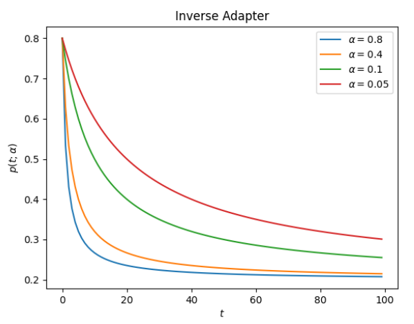
The Inverse Adapter uses the following form to change the initial value:

This formula requires that alpha is in the range (0, 1) to have the desired properties. This is how the adapter looks:

As we saw, all the adapters change the initial parameter at a different rate (which depends on alpha), so it’s helpful to see how they behave in comparison; this is the result for a fixed alpha value of 0.15.
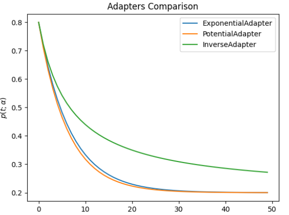
You can see that the potential adapter is the one that decreases more rapidly, followed very close by the exponential; the inverse adapter may require a longer number of iterations to converge.
This is the code used for this comparison in case you want to play with the parameters to see its effect; first, make sure to install the package:
pip install sklearn-genetic-opt
In this section, we want to use an algorithm for automatic hyperparameter tuning; such algorithms usually come with options to control de optimization process; for example, I’m going to use a genetic algorithm to control the mutation and crossover probabilities with an exponential adapter; these are related to the exploration vs. exploration strategy of the algorithm.
You can check this other article I wrote to understand more about genetic algorithms for hyperparameter tuning.
First, let us import the package we require. I will use the digits dataset and fine-tune a Random Forest model.
Note: I’m the author of the package used in the example; if you want to know further, contribute or make some suggestions, you can check the documentation and the GitHub repository at the end of this article.
The para_grid parameter delimits the model’s hyperparameters search space and defines the data types; we’ll use the cross-validation accuracy to evaluate the model’s hyperparameters.
We define the optimization algorithm and create the adaptive crossover and mutation probabilities. We’ll start with a high mutation probability and a low crossover probability; as the generations increase, the crossover and mutation probability will increase and decrease, respectively.
We’ll also print and plot some statistics to understand the results.
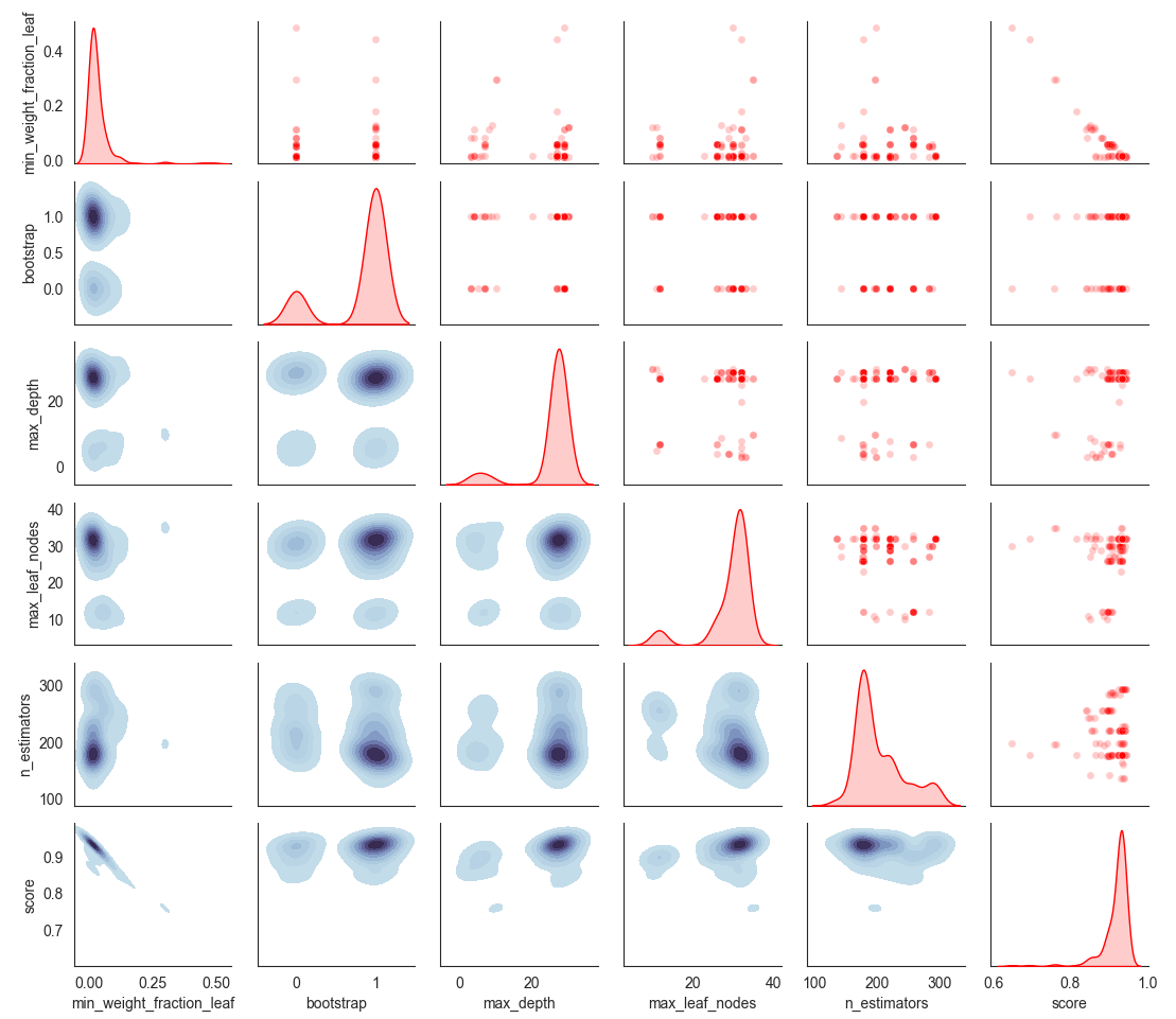
In this particular example, I got an accuracy score of 0.941 (on test data) and found these parameters:
{‘min_weight_fraction_leaf’: 0.01079845233781555, ‘bootstrap’: True, ‘max_depth’: 10, ‘max_leaf_nodes’: 27, ‘n_estimators’: 108}
You can check the search space, which shows which hyperparameters were explored by the algorithm.

For reference, this is how the sampled space looks without adaptive learning; the algorithm explored fewer regions with a fixed low mutation probability (0.2) and a high crossover probability (0.8).
Adapting or scheduling parameters can be very useful when training a machine learning algorithm; it might allow you to converge the algorithm faster or to explore complex regions of space with a dynamic strategy, even if the literature mainly uses them for deep learning, as we’ve shown, you can also use this for traditional machine learning, and adapt its ideas to extend it to any other set of problems that may suit a changing parameter strategy.
If you want to know more about sklearn-genetic-opt, you can check the documentation here:
Let’s explore some methods to adapt your parameters over time.

In this post, I will discuss the ideas behind adaptive parameters methods for machine learning and why and when to implement them as some practical examples using python.
Adaptive methods (also known as parameter scheduling) refer to strategies to update some model parameters at training time using a schedule.
This change will depend on the model’s state at time t; for example, you can set update them depending on the loss value, the number of iterations/epochs, elapsed training time, etc.
For example, in general, for neural networks, the choice of the learning rate has several consequences; if the learning rate is too large, it may overshoot the minimum; if it’s too small, it may take it too long to converge, or it might get stuck on a local minimum.
In this scenario, we choose to change the learning rate as a function of the epochs; this way, you may set a large rate at the beginning of the training, and conforming to the epochs increases; you can decrease the value until you reach a lower threshold.
You can also see it as a way of exploration vs. exploitation strategy, so at the beginning, you allow more exploration, and at the end, you choose exploitation.
There are several methods you can choose to control the form and the speed from which the parameter goes from an initial value to a final threshold; in this article, I’ll call them “Adapters”, and I’ll focus on methods that change the parameter value as a function of the number of iterations (epochs in case of neural networks).
I’ll introduce some definitions and notation:
The initial value represents the starting point of the parameter, the end_value is the value you’d get after many iterations, and the adaptive rate controls how fast you go from the initial_value to the end_value.
Under this scenario, you would expect to have the following properties for each adapter:
In this article, I’ll explain three types of adapters:
- Exponential
- Inverse
- Potential
The Exponential Adapter uses the following form to change the initial value:
From this formula, alpha should be a positive value to have the desired properties.
If we plot this adapter for different alpha values, we can see how the parameter value decreases with different shapes, but all of them follow an exponential decay; this shows how the choice of alpha affects the decay speed.
In this example, the initial_value is 0.8, and the end value is 0.2. You can see that larger alpha values require fewer steps/iterations to converge to a value close to 0.2.
If you select the initial_value to be lower than the end_value, you’ll be performing an exponential ascend, which can be helpful in some cases; for example, in genetic algorithms, you may start with a low crossover probability at the first generation, and increase it as the generations go forward.
The following is how the above plot would look if the starting point is 0.2 and goes until 0.8; you can see the symmetry against the decay.
The Inverse Adapter uses the following form to change the initial value:
From this formula, alpha should be a positive value to have the desired properties. This is how the adapter looks:
The Inverse Adapter uses the following form to change the initial value:
This formula requires that alpha is in the range (0, 1) to have the desired properties. This is how the adapter looks:
As we saw, all the adapters change the initial parameter at a different rate (which depends on alpha), so it’s helpful to see how they behave in comparison; this is the result for a fixed alpha value of 0.15.
You can see that the potential adapter is the one that decreases more rapidly, followed very close by the exponential; the inverse adapter may require a longer number of iterations to converge.
This is the code used for this comparison in case you want to play with the parameters to see its effect; first, make sure to install the package:
pip install sklearn-genetic-opt
In this section, we want to use an algorithm for automatic hyperparameter tuning; such algorithms usually come with options to control de optimization process; for example, I’m going to use a genetic algorithm to control the mutation and crossover probabilities with an exponential adapter; these are related to the exploration vs. exploration strategy of the algorithm.
You can check this other article I wrote to understand more about genetic algorithms for hyperparameter tuning.
First, let us import the package we require. I will use the digits dataset and fine-tune a Random Forest model.
Note: I’m the author of the package used in the example; if you want to know further, contribute or make some suggestions, you can check the documentation and the GitHub repository at the end of this article.
The para_grid parameter delimits the model’s hyperparameters search space and defines the data types; we’ll use the cross-validation accuracy to evaluate the model’s hyperparameters.
We define the optimization algorithm and create the adaptive crossover and mutation probabilities. We’ll start with a high mutation probability and a low crossover probability; as the generations increase, the crossover and mutation probability will increase and decrease, respectively.
We’ll also print and plot some statistics to understand the results.
In this particular example, I got an accuracy score of 0.941 (on test data) and found these parameters:
{‘min_weight_fraction_leaf’: 0.01079845233781555, ‘bootstrap’: True, ‘max_depth’: 10, ‘max_leaf_nodes’: 27, ‘n_estimators’: 108}
You can check the search space, which shows which hyperparameters were explored by the algorithm.
For reference, this is how the sampled space looks without adaptive learning; the algorithm explored fewer regions with a fixed low mutation probability (0.2) and a high crossover probability (0.8).
Adapting or scheduling parameters can be very useful when training a machine learning algorithm; it might allow you to converge the algorithm faster or to explore complex regions of space with a dynamic strategy, even if the literature mainly uses them for deep learning, as we’ve shown, you can also use this for traditional machine learning, and adapt its ideas to extend it to any other set of problems that may suit a changing parameter strategy.
If you want to know more about sklearn-genetic-opt, you can check the documentation here:
Denial of responsibility! Techno Blender is an automatic aggregator of the all world’s media. In each content, the hyperlink to the primary source is specified. All trademarks belong to their rightful owners, all materials to their authors. If you are the owner of the content and do not want us to publish your materials, please contact us by email – [email protected]. The content will be deleted within 24 hours.