
All You Need to Know About Bag of Words and Word2Vec — Text Feature Extraction | by Albers Uzila | Aug, 2022
Data Science
Why Word2Vec is better, and why it’s not good enough
While image data is straightforward to be used by deep learning models (RGB value as the input), this is not the case for text data. Deep learning models only work on numbers, not sequences of symbols like texts. So, you need a way to somehow extract meaningful numerical feature vectors from texts. This is called feature extraction.
From now on, we will call a single observation of text by document and a collection of documents by corpus.
Table of Contents· Bag of Words
∘ The Basics
∘ Example on Data
∘ Advantages & Limitations· Word2Vec
∘ The Basics
∘ Creating Train Data
∘ Continuous Bag of Words & Skip-Gram
∘ Advantages & Limitations· Summary
The Basics
One of the most intuitive features to create is the number of times each word appears in a document. So, what you need to do is:
- Tokenize each document and give an integer id for each token. The token separators could be white spaces and punctuation.
- Count the occurrences of tokens in each document.
The number of occurrences of tokens is called term frequency (tf). Albeit simple, term frequencies are not necessarily the best corpus representation. According to Zipf’s law, common words like “the”, “a”, and “to” are almost always the terms/tokens with the highest frequency in the document. If you were to feed the term frequencies directly to a classifier, those very frequent tokens would shadow the frequencies of rarer yet more interesting tokens.
To address this problem, one of the most popular ways to “normalize” term frequencies is to weight each token by the inverse of document frequency (idf), which is given by

where m is the total number of documents in the corpus, and df(t) is the number of documents in the corpus that contain token t. The weighted tf is named tf-idf and is given by

for a token t of document d in the corpus. The Euclidean norm then normalizes the resulting tf-idf vectors, i.e.,

for any tf-idf vector v.
Example on Data
As a concrete example, let’s say you have the following corpus.
corpus = [
'This is the first document.',
'This is the second second document.',
'And the third one.',
'Is this the first document?',
]
Then, m = 4. After tokenizing, there are 9 tokens in the corpus in total: ‘and’, ‘document’, ‘first’, ‘is’, ‘one’, ‘second’, ‘the’, ‘third’, and ‘this’. So, term frequencies can be represented as a matrix of size 4×9:

df(t) can then be calculated from term frequencies by counting the number of non-zero values for each token, and idf(t) is calculated using the formula above:

tf-idf(t, d) is obtained by multiplying the tf matrix above with idf for each token.

For each document, respectively, the Euclidean norm of tf-idf is displayed below.
2.97, 5.36, 4.25, 2.97
Then, the normalized tf-idf is calculated by dividing the original tf-idf with the appropriate Euclidean norm for each document. You obtain the normalized tf-idf as follows.

These are the final features to be fed into a model.
Advantages & Limitations
Since every word is represented by a scalar, the bag of words representation of texts is very lightweight and easily understood. Nevertheless, it suffers at least 2 significant disadvantages:
- The feature dimension is linearly dependent on the number of unique tokens (let’s call it
vocab_size) which is bad news when you have a large corpus. You could discard a few least occurring tokens to save space but then you’d throw away some potentially useful information from the data. - If you look at the first and the last document from the above example on data, you’ll realize that they are different documents yet have the same feature vector. This is because the bag of words doesn’t preserve relationships between tokens.
To address limitation 2, you could add n-grams as new features, which capture n consecutive tokens (and hence their relationships). However, this leads again to limitation 1 where you’d need to save extra space for the extra features.
The Basics
Word2Vec addresses both limitations of the bag of words representation simultaneously:
- Instead of having a feature vector for each document with a length equals
vocab_size, now each token becomes a vector with the length of a number you determine (typically 100–1000, let’s call itembed_dim). - Instead of vectorizing a token itself, Word2Vec vectorizes the context of the token by considering neighboring tokens.
The result is a vocab_size × embed_dim matrix. So, how does Word2Vec learn the context of a token?
Note: Before continuing, it’s good to know what a dense neural network and activation function is. Here’s a story for that.
Word2Vec employs the use of a dense neural network with a single hidden layer that has no activation function, that predicts a one-hot encoded token given another one-hot encoded token.
The input layer has vocab_size neurons, the hidden layer has embed_dim neurons, and the output layer also has vocab_size neurons. The output layer is passed through the softmax activation function that treats the problem as multiclass.
Below is the architecture of the network, where xᵢ ∈ {0, 1} after one-hot encoding the tokens, ∑ represents the weighted sum of the output of the previous layer, and S means softmax.

The weight matrix associated with the hidden layer from the input layer is called word embedding and has the dimension vocab_size × embed_dim. When you use it in your NLP tasks, it acts as a lookup table to convert words to vectors (hence the name). At the end of the training Word2Vec, you throw away everything except the word embedding.
You have the neural network model. Now, how about the train data?
Creating Train Data
Creating data to train the neural network involves assigning every word to be a center word and its neighboring words to be the context words. The number of the neighboring words is defined by a window, a hyperparameter.
To be concrete, let’s go back to our previous example. We will use window = 1 (1 context word for each left and right of the center word). The process of generating train data can be seen below.

Words colored in green are the center words, and those colored in orange are the context words. One word at a time, you’re creating (center, context) pairs. Repeat this for every document in the corpus.
The idea of Word2Vec is that similar center words will appear with similar contexts and you can learn this relationship by repeatedly training your model with (center, context) pairs.
Continuous Bag of Words & Skip-Gram
There are two ways Word2Vec learns the context of tokens. The difference between the two is the input data and labels used.
1. Continuous Bag of Words (CBOW)
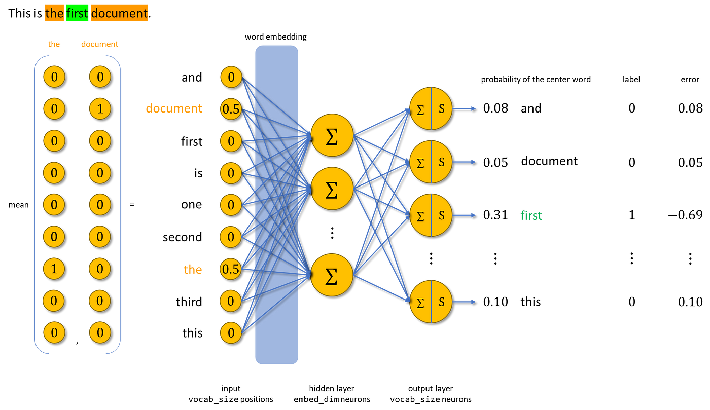
Given context words, CBOW will take the average of their one-hot encoding and predict the one-hot encoding of the center word. The diagram below explains this process.
2. Skip-Gram (SG)
Given a center word, SG will one-hot encode it and maximize the probabilities of the context words at the output. The error is calculated for each context word and then summed up. Below is the training process.

Since softmax is used to compute the probability distribution of all words in the output layer (which could be millions or more), the training process is very computationally expensive.
To address this issue, you could reformulate the problem as a set of independent binary classification tasks and use negative sampling. The new objective is to predict, for any given (word, context) pair, whether the word is in the context window of the center word or not.
Negative sampling only updates the correct class and a few arbitrary (a hyperparameter) incorrect classes. We’re able to do this because of the large amount of train data where we’ll see the same word as the target class multiple times.
Advantages & Limitations
SG works well with a small amount of train data and represents infrequent words or phrases well. But this comes at the price of increased computational cost.
CBOW is several times faster to train than SG with slightly better accuracy for frequent words. If training time is a big concern and you have large enough data to overcome the issue of predicting infrequent words, CBOW may be a more viable choice.
Since there’s only a linear relationship between the input layer to the output layer (before softmax), the feature vectors produced by Word2Vec can be linearly related. For example, vec(king) – vec(man) + vec(woman) ≈ vec(queen), which kind of makes sense for our little mushy human brain.
Yet, there are still some limitations to Word2Vec, four of which are:
- Word2Vec relies on local information about words, i.e. the context of a word relies only on its neighbors.
- Word embedding is a byproduct of training a neural network, hence the linear relationships between feature vectors are a black box (kind of).
- Word2Vec cannot understand out-of-vocabulary (OOV) words, i.e. words not present in train data. You could assign a UNK token which is used for all OOV words or you could use other models that are robust to OOV words.
- By assigning a distinct vector to each word, Word2Vec ignores the morphology of words. For example, eat, eats, and eaten are considered independently different words by Word2Vec, but they come from the same root: eat. This information might be useful.
In the next story, we will propose and explain embedding models that in theory could resolve these limitations. Stay tuned!
Thanks for reaching the end!
In this story, you are introduced to 2 methods that can extract features from text data:
- Bag of words tokenizes each document and counts the occurrences of each token.
- Word2Vec employs the use of a dense neural network with a single hidden layer to learn word embedding from one-hot encoded words.
While the bag of words is simple, it doesn’t capture the relationships between tokens and the feature dimension obtained becomes really big for a large corpus. Word2Vec addresses this issue by using (center, context) word pairs and allowing us to customize the length of feature vectors.
However, Word2Vec is not perfect. It cannot understand OOV words and ignores the morphology of words.
Data Science
Why Word2Vec is better, and why it’s not good enough

While image data is straightforward to be used by deep learning models (RGB value as the input), this is not the case for text data. Deep learning models only work on numbers, not sequences of symbols like texts. So, you need a way to somehow extract meaningful numerical feature vectors from texts. This is called feature extraction.
From now on, we will call a single observation of text by document and a collection of documents by corpus.
Table of Contents· Bag of Words
∘ The Basics
∘ Example on Data
∘ Advantages & Limitations· Word2Vec
∘ The Basics
∘ Creating Train Data
∘ Continuous Bag of Words & Skip-Gram
∘ Advantages & Limitations· Summary
The Basics
One of the most intuitive features to create is the number of times each word appears in a document. So, what you need to do is:
- Tokenize each document and give an integer id for each token. The token separators could be white spaces and punctuation.
- Count the occurrences of tokens in each document.
The number of occurrences of tokens is called term frequency (tf). Albeit simple, term frequencies are not necessarily the best corpus representation. According to Zipf’s law, common words like “the”, “a”, and “to” are almost always the terms/tokens with the highest frequency in the document. If you were to feed the term frequencies directly to a classifier, those very frequent tokens would shadow the frequencies of rarer yet more interesting tokens.
To address this problem, one of the most popular ways to “normalize” term frequencies is to weight each token by the inverse of document frequency (idf), which is given by
where m is the total number of documents in the corpus, and df(t) is the number of documents in the corpus that contain token t. The weighted tf is named tf-idf and is given by
for a token t of document d in the corpus. The Euclidean norm then normalizes the resulting tf-idf vectors, i.e.,
for any tf-idf vector v.
Example on Data
As a concrete example, let’s say you have the following corpus.
corpus = [
'This is the first document.',
'This is the second second document.',
'And the third one.',
'Is this the first document?',
]
Then, m = 4. After tokenizing, there are 9 tokens in the corpus in total: ‘and’, ‘document’, ‘first’, ‘is’, ‘one’, ‘second’, ‘the’, ‘third’, and ‘this’. So, term frequencies can be represented as a matrix of size 4×9:
df(t) can then be calculated from term frequencies by counting the number of non-zero values for each token, and idf(t) is calculated using the formula above:
tf-idf(t, d) is obtained by multiplying the tf matrix above with idf for each token.
For each document, respectively, the Euclidean norm of tf-idf is displayed below.
2.97, 5.36, 4.25, 2.97
Then, the normalized tf-idf is calculated by dividing the original tf-idf with the appropriate Euclidean norm for each document. You obtain the normalized tf-idf as follows.
These are the final features to be fed into a model.
Advantages & Limitations
Since every word is represented by a scalar, the bag of words representation of texts is very lightweight and easily understood. Nevertheless, it suffers at least 2 significant disadvantages:
- The feature dimension is linearly dependent on the number of unique tokens (let’s call it
vocab_size) which is bad news when you have a large corpus. You could discard a few least occurring tokens to save space but then you’d throw away some potentially useful information from the data. - If you look at the first and the last document from the above example on data, you’ll realize that they are different documents yet have the same feature vector. This is because the bag of words doesn’t preserve relationships between tokens.
To address limitation 2, you could add n-grams as new features, which capture n consecutive tokens (and hence their relationships). However, this leads again to limitation 1 where you’d need to save extra space for the extra features.
The Basics
Word2Vec addresses both limitations of the bag of words representation simultaneously:
- Instead of having a feature vector for each document with a length equals
vocab_size, now each token becomes a vector with the length of a number you determine (typically 100–1000, let’s call itembed_dim). - Instead of vectorizing a token itself, Word2Vec vectorizes the context of the token by considering neighboring tokens.
The result is a vocab_size × embed_dim matrix. So, how does Word2Vec learn the context of a token?
Note: Before continuing, it’s good to know what a dense neural network and activation function is. Here’s a story for that.
Word2Vec employs the use of a dense neural network with a single hidden layer that has no activation function, that predicts a one-hot encoded token given another one-hot encoded token.
The input layer has vocab_size neurons, the hidden layer has embed_dim neurons, and the output layer also has vocab_size neurons. The output layer is passed through the softmax activation function that treats the problem as multiclass.
Below is the architecture of the network, where xᵢ ∈ {0, 1} after one-hot encoding the tokens, ∑ represents the weighted sum of the output of the previous layer, and S means softmax.
The weight matrix associated with the hidden layer from the input layer is called word embedding and has the dimension vocab_size × embed_dim. When you use it in your NLP tasks, it acts as a lookup table to convert words to vectors (hence the name). At the end of the training Word2Vec, you throw away everything except the word embedding.
You have the neural network model. Now, how about the train data?
Creating Train Data
Creating data to train the neural network involves assigning every word to be a center word and its neighboring words to be the context words. The number of the neighboring words is defined by a window, a hyperparameter.
To be concrete, let’s go back to our previous example. We will use window = 1 (1 context word for each left and right of the center word). The process of generating train data can be seen below.
Words colored in green are the center words, and those colored in orange are the context words. One word at a time, you’re creating (center, context) pairs. Repeat this for every document in the corpus.
The idea of Word2Vec is that similar center words will appear with similar contexts and you can learn this relationship by repeatedly training your model with (center, context) pairs.
Continuous Bag of Words & Skip-Gram
There are two ways Word2Vec learns the context of tokens. The difference between the two is the input data and labels used.
1. Continuous Bag of Words (CBOW)
Given context words, CBOW will take the average of their one-hot encoding and predict the one-hot encoding of the center word. The diagram below explains this process.
2. Skip-Gram (SG)
Given a center word, SG will one-hot encode it and maximize the probabilities of the context words at the output. The error is calculated for each context word and then summed up. Below is the training process.
Since softmax is used to compute the probability distribution of all words in the output layer (which could be millions or more), the training process is very computationally expensive.
To address this issue, you could reformulate the problem as a set of independent binary classification tasks and use negative sampling. The new objective is to predict, for any given (word, context) pair, whether the word is in the context window of the center word or not.
Negative sampling only updates the correct class and a few arbitrary (a hyperparameter) incorrect classes. We’re able to do this because of the large amount of train data where we’ll see the same word as the target class multiple times.
Advantages & Limitations
SG works well with a small amount of train data and represents infrequent words or phrases well. But this comes at the price of increased computational cost.
CBOW is several times faster to train than SG with slightly better accuracy for frequent words. If training time is a big concern and you have large enough data to overcome the issue of predicting infrequent words, CBOW may be a more viable choice.
Since there’s only a linear relationship between the input layer to the output layer (before softmax), the feature vectors produced by Word2Vec can be linearly related. For example, vec(king) – vec(man) + vec(woman) ≈ vec(queen), which kind of makes sense for our little mushy human brain.
Yet, there are still some limitations to Word2Vec, four of which are:
- Word2Vec relies on local information about words, i.e. the context of a word relies only on its neighbors.
- Word embedding is a byproduct of training a neural network, hence the linear relationships between feature vectors are a black box (kind of).
- Word2Vec cannot understand out-of-vocabulary (OOV) words, i.e. words not present in train data. You could assign a UNK token which is used for all OOV words or you could use other models that are robust to OOV words.
- By assigning a distinct vector to each word, Word2Vec ignores the morphology of words. For example, eat, eats, and eaten are considered independently different words by Word2Vec, but they come from the same root: eat. This information might be useful.
In the next story, we will propose and explain embedding models that in theory could resolve these limitations. Stay tuned!
Thanks for reaching the end!
In this story, you are introduced to 2 methods that can extract features from text data:
- Bag of words tokenizes each document and counts the occurrences of each token.
- Word2Vec employs the use of a dense neural network with a single hidden layer to learn word embedding from one-hot encoded words.
While the bag of words is simple, it doesn’t capture the relationships between tokens and the feature dimension obtained becomes really big for a large corpus. Word2Vec addresses this issue by using (center, context) word pairs and allowing us to customize the length of feature vectors.
However, Word2Vec is not perfect. It cannot understand OOV words and ignores the morphology of words.
Denial of responsibility! Techno Blender is an automatic aggregator of the all world’s media. In each content, the hyperlink to the primary source is specified. All trademarks belong to their rightful owners, all materials to their authors. If you are the owner of the content and do not want us to publish your materials, please contact us by email – [email protected]. The content will be deleted within 24 hours.