
An Introduction to Air Travel Network Optimization Using Mixed Integer Programming
How to design an algorithm to route passenger demand across a network in the most cost-effective manner
Introduction:
This is a take on the Vehicle Routing Problem problem, but adapted to the air transport networks, namely the Origin Destination-to-Leg problem.
A little background first: Airlines are constantly faced with the question of how to address demand between city-pairs — do they open a direct connection, or provide connecting itineraries so that the demand is channeled through one or more hubs? The latter is of course preferable from a passenger perspective, but is more costly for the airline and therefore riskier — what if the flight is not filled? Operating a route is very expensive. In other words, we are trying to do this*:
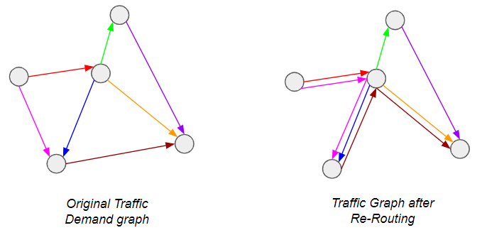
*Graph theory enthusiasts will recognize this as a special case of the Graph Sparsification problem, which has seen considerable attention lately.
The industry typically addresses this using so-called itinerary choice models, which are simply probabilistic models to determine which routings passengers will prefer on the basis of number of connections, route length, flight times etc… While this works well when the network shape is already fixed, deciding which routes to open is more complicated. This is because there are a number of routes which are only viable if they can capture enough connecting traffic from other sources — this in turn only occurs if there are no direct routes to serve said traffic. In other words, the status of each route is dependent on the status of neighboring routes, turning this into a combinatorial problem.
This is precisely the kind of problem that Mixed Integer Programs (MIP) are designed for! Specifically, we will formulate a problem to reflect the following behaviors: Network Flow Conservation and Edge Activation Costs to enforce sparsification.
Toy Problem:
For the rest of this article, I will use a toy example as illustration. To completely describe the problem, we need the following inputs:
Input Graph:
A dense Origin-Destination bidirectional graph G = (V, E), with n vertices V and m edges E. Each edge has as attribute the Origin-Destination demand (O) and the distance between each city-pair (Distance). Typically, the demand follows a pareto distribution, where a few edges have high demand and the rest have low demand*:

*Graph generated by randomly instantiating the coordinates of the nodes and their population. Using the so-called gravity model for transport, a realistic demand profile can then be obtained. For more information, see link
Cost Assumptions:
Depending on the edge distance and typical vehicle type that would be assigned, each edge would have the following cost properties:
- Cost of per passenger, Costₚₐₓ, where pax is short-hand for passenger. In practice, it is the cost-per-seat that should be considered, rather than cost-per-pax, since not every vehicle is necessarily filled completely. However, this would require discrete modelling of each vehicle (and an associated integer variable), which would explode the size of the problem.
- Minimum cost of operating a route, Costₘᵢₙ. Think of this as the edge activation cost.
Bear in mind that both Costₚₐₓ and Costₘᵢₙ are m × 1 vectors (one per edge), and both costs scale linearly with distance.
With this, we have everything we need to design our MIP. As you might have guessed, the idea is to minimize the cost function of the system while respecting the network flow constraint.
Network Flow Conservation
This is a well-known condition, which states that the inflow and outflow of each vertex must be balanced, unless it is a source or sink:
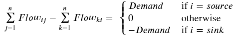
Here (i, j, k) are vertex indices. I’m personally not a big fan of this type of notation, and prefer the equivalent expression using the concept of the edge-incidence matrix from graph theory. This is usually denoted by the n × m matrix B, where each row entry is zero except at the incidence vertices for the corresponding edge, which are 1 & -1 to represent the source & sink:

If we initialize an m × m variable matrix (let’s call it R for Itinerary Routing — see Figure 1) to represent the flow routing for each demand edge in G, we can equivalently formulate the above condition by:
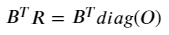
Where diag(O) is an m × m matrix with each diagonal entry corresponding to the demand from edge i. If you multiply out any row i of the RHS, it immediately becomes obvious why any R that satisfies this equation is valid from a flow conservation perspective.
Note however that both the B and R are directional. In the context of our cost function, we don’t really care whether some flows are negative — we just want the absolute, total number of passengers flowing along the edge i in order to quantify the cost of carrying them. To represent this, we can define the m × 1 leg vector L:

With these definitions, we have a function mapping O → L that is compatible with the network flow conservation principle. From hereon, L represents the total passenger volume on each edge.
Edge Activation
This is the heart of the problem! Consider that if Costₘᵢₙ=0, the solution would be trivial, with L mapping to O on a one-to-one basis. This is because any alternative routing would necessarily cover a longer distance than the direct route, so that the cheapest option would always be the latter. However, in the presence of Costₘᵢₙ, there is a trade-off between the △Cost incurred by longer distance travelled vs. △Cost incurred through edge-activation. In other words, we need the cost profile for each edge to be:
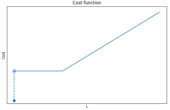
There are 3 parts to this function:
- If the number of passengers is zero, no costs are incurred (Cost = 0)
- If the number of passengers is between 0 and the threshold, a fixed cost is incurred (Cost = Cₘᵢₙ), no matter the number of passengers.
- If the number of passengers exceeds the threshold, costs scale linearly with according to the cost per pax (Cost = Cₚₐₓ.L)
If it were not for the zero-point discontinuity, this would have been a pretty simple problem to solve. Instead, we have a non-convex, combinatorial problem because there is a sudden shift in behavior depending on whether the number of passengers along an edge is zero or not. In this situation, we need an activation (binary) variable to tell the algorithm which condition to follow. Using the big-M approach, we can formulate this as follows:

Where the m × 1 vector of binary variables z (i.e. z ∈ [0,1]) indicates if a route is open or not, and a very large scalar variable M. If you’re not familiar with the big-M method, you can read up on it here. In this context, it simply enforces the following conditions:
- Lᵢ = 0 → zᵢ=0
- Lᵢ >0 → zᵢ=1
Ideally, we would have liked to simply multiply the cost function by this activation variable to tell it which cost behavior to follow. However, this would make the constraint non-linear and very complicated to solve. Instead, we can use Big-M again, this time to linearize the problem while getting the same effect:
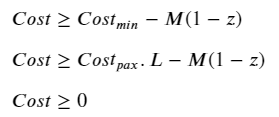
Combining the cost minimization objective with the ≥ inequalities, we basically end up with a minmax problem where:
- zᵢ=0 → Costᵢ = minmax(0, -M) = 0.
- zᵢ=1 → Costᵢ = minmax(Cₘᵢₙ, CₚₐₓL).
And there we have it! The complete formulation of the problem is shown:
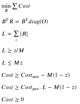
We now only have to plug in some numbers to see the magic happen.
Sensitivity to minimum threshold
It should be clear from the description that the minimum threshold is the main input of interest here, because it defines the degree of sparsification. It’s interesting to see the impact using progressively higher thresholds:
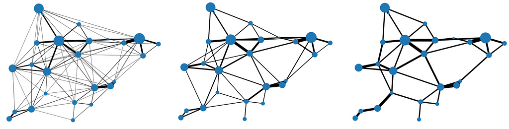
Notice how, no matter the threshold, the graph remains connected — this is a result of the network flow conservation principle, to ensure all demand is satisfied. Another neat way to visualize it is to look at the demand distribution along edges:
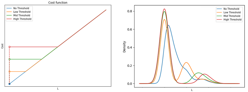
Here we see how the higher the threshold, the higher the level of consolidation (fewer routes with higher volume of traffic), and a correspondingly high number of routes with no traffic.
Conclusion
This was a simple introduction to what is in reality a very complex problem (there is far more nuance to airline networks than just minimum threshold costs). Still, it demonstrates one of the core behaviors of real networks, while giving a basic introduction to some key concepts for formulating MIPs. The codes for this are on my Github, feel free to give it a try.
If you actually try to run it, you’ll soon notice that solve time scales exponentially with the number of vertices in the graph. This is especially the case if you solve it with cvxpy — a common (but rudimentary) open source python library for simple optimization problems. That said, even the sophisticated commercial solvers soon run into their limits. This is the unescapable truth of combinatorial problems; they scale poorly, and are often impractical beyond a certain problem size.
In the next article, I will introduce a way to try to abstract away some of the complexity by using Graph Neural Networks as surrogate models.
All images unless otherwise stated are by me, the author.
An Introduction to Air Travel Network Optimization Using Mixed Integer Programming was originally published in Towards Data Science on Medium, where people are continuing the conversation by highlighting and responding to this story.
How to design an algorithm to route passenger demand across a network in the most cost-effective manner
Introduction:
This is a take on the Vehicle Routing Problem problem, but adapted to the air transport networks, namely the Origin Destination-to-Leg problem.

A little background first: Airlines are constantly faced with the question of how to address demand between city-pairs — do they open a direct connection, or provide connecting itineraries so that the demand is channeled through one or more hubs? The latter is of course preferable from a passenger perspective, but is more costly for the airline and therefore riskier — what if the flight is not filled? Operating a route is very expensive. In other words, we are trying to do this*:
*Graph theory enthusiasts will recognize this as a special case of the Graph Sparsification problem, which has seen considerable attention lately.
The industry typically addresses this using so-called itinerary choice models, which are simply probabilistic models to determine which routings passengers will prefer on the basis of number of connections, route length, flight times etc… While this works well when the network shape is already fixed, deciding which routes to open is more complicated. This is because there are a number of routes which are only viable if they can capture enough connecting traffic from other sources — this in turn only occurs if there are no direct routes to serve said traffic. In other words, the status of each route is dependent on the status of neighboring routes, turning this into a combinatorial problem.
This is precisely the kind of problem that Mixed Integer Programs (MIP) are designed for! Specifically, we will formulate a problem to reflect the following behaviors: Network Flow Conservation and Edge Activation Costs to enforce sparsification.
Toy Problem:
For the rest of this article, I will use a toy example as illustration. To completely describe the problem, we need the following inputs:
Input Graph:
A dense Origin-Destination bidirectional graph G = (V, E), with n vertices V and m edges E. Each edge has as attribute the Origin-Destination demand (O) and the distance between each city-pair (Distance). Typically, the demand follows a pareto distribution, where a few edges have high demand and the rest have low demand*:
*Graph generated by randomly instantiating the coordinates of the nodes and their population. Using the so-called gravity model for transport, a realistic demand profile can then be obtained. For more information, see link
Cost Assumptions:
Depending on the edge distance and typical vehicle type that would be assigned, each edge would have the following cost properties:
- Cost of per passenger, Costₚₐₓ, where pax is short-hand for passenger. In practice, it is the cost-per-seat that should be considered, rather than cost-per-pax, since not every vehicle is necessarily filled completely. However, this would require discrete modelling of each vehicle (and an associated integer variable), which would explode the size of the problem.
- Minimum cost of operating a route, Costₘᵢₙ. Think of this as the edge activation cost.
Bear in mind that both Costₚₐₓ and Costₘᵢₙ are m × 1 vectors (one per edge), and both costs scale linearly with distance.
With this, we have everything we need to design our MIP. As you might have guessed, the idea is to minimize the cost function of the system while respecting the network flow constraint.
Network Flow Conservation
This is a well-known condition, which states that the inflow and outflow of each vertex must be balanced, unless it is a source or sink:
Here (i, j, k) are vertex indices. I’m personally not a big fan of this type of notation, and prefer the equivalent expression using the concept of the edge-incidence matrix from graph theory. This is usually denoted by the n × m matrix B, where each row entry is zero except at the incidence vertices for the corresponding edge, which are 1 & -1 to represent the source & sink:
If we initialize an m × m variable matrix (let’s call it R for Itinerary Routing — see Figure 1) to represent the flow routing for each demand edge in G, we can equivalently formulate the above condition by:
Where diag(O) is an m × m matrix with each diagonal entry corresponding to the demand from edge i. If you multiply out any row i of the RHS, it immediately becomes obvious why any R that satisfies this equation is valid from a flow conservation perspective.
Note however that both the B and R are directional. In the context of our cost function, we don’t really care whether some flows are negative — we just want the absolute, total number of passengers flowing along the edge i in order to quantify the cost of carrying them. To represent this, we can define the m × 1 leg vector L:
With these definitions, we have a function mapping O → L that is compatible with the network flow conservation principle. From hereon, L represents the total passenger volume on each edge.
Edge Activation
This is the heart of the problem! Consider that if Costₘᵢₙ=0, the solution would be trivial, with L mapping to O on a one-to-one basis. This is because any alternative routing would necessarily cover a longer distance than the direct route, so that the cheapest option would always be the latter. However, in the presence of Costₘᵢₙ, there is a trade-off between the △Cost incurred by longer distance travelled vs. △Cost incurred through edge-activation. In other words, we need the cost profile for each edge to be:
There are 3 parts to this function:
- If the number of passengers is zero, no costs are incurred (Cost = 0)
- If the number of passengers is between 0 and the threshold, a fixed cost is incurred (Cost = Cₘᵢₙ), no matter the number of passengers.
- If the number of passengers exceeds the threshold, costs scale linearly with according to the cost per pax (Cost = Cₚₐₓ.L)
If it were not for the zero-point discontinuity, this would have been a pretty simple problem to solve. Instead, we have a non-convex, combinatorial problem because there is a sudden shift in behavior depending on whether the number of passengers along an edge is zero or not. In this situation, we need an activation (binary) variable to tell the algorithm which condition to follow. Using the big-M approach, we can formulate this as follows:
Where the m × 1 vector of binary variables z (i.e. z ∈ [0,1]) indicates if a route is open or not, and a very large scalar variable M. If you’re not familiar with the big-M method, you can read up on it here. In this context, it simply enforces the following conditions:
- Lᵢ = 0 → zᵢ=0
- Lᵢ >0 → zᵢ=1
Ideally, we would have liked to simply multiply the cost function by this activation variable to tell it which cost behavior to follow. However, this would make the constraint non-linear and very complicated to solve. Instead, we can use Big-M again, this time to linearize the problem while getting the same effect:
Combining the cost minimization objective with the ≥ inequalities, we basically end up with a minmax problem where:
- zᵢ=0 → Costᵢ = minmax(0, -M) = 0.
- zᵢ=1 → Costᵢ = minmax(Cₘᵢₙ, CₚₐₓL).
And there we have it! The complete formulation of the problem is shown:
We now only have to plug in some numbers to see the magic happen.
Sensitivity to minimum threshold
It should be clear from the description that the minimum threshold is the main input of interest here, because it defines the degree of sparsification. It’s interesting to see the impact using progressively higher thresholds:
Notice how, no matter the threshold, the graph remains connected — this is a result of the network flow conservation principle, to ensure all demand is satisfied. Another neat way to visualize it is to look at the demand distribution along edges:
Here we see how the higher the threshold, the higher the level of consolidation (fewer routes with higher volume of traffic), and a correspondingly high number of routes with no traffic.
Conclusion
This was a simple introduction to what is in reality a very complex problem (there is far more nuance to airline networks than just minimum threshold costs). Still, it demonstrates one of the core behaviors of real networks, while giving a basic introduction to some key concepts for formulating MIPs. The codes for this are on my Github, feel free to give it a try.
If you actually try to run it, you’ll soon notice that solve time scales exponentially with the number of vertices in the graph. This is especially the case if you solve it with cvxpy — a common (but rudimentary) open source python library for simple optimization problems. That said, even the sophisticated commercial solvers soon run into their limits. This is the unescapable truth of combinatorial problems; they scale poorly, and are often impractical beyond a certain problem size.
In the next article, I will introduce a way to try to abstract away some of the complexity by using Graph Neural Networks as surrogate models.
All images unless otherwise stated are by me, the author.
An Introduction to Air Travel Network Optimization Using Mixed Integer Programming was originally published in Towards Data Science on Medium, where people are continuing the conversation by highlighting and responding to this story.
Denial of responsibility! Techno Blender is an automatic aggregator of the all world’s media. In each content, the hyperlink to the primary source is specified. All trademarks belong to their rightful owners, all materials to their authors. If you are the owner of the content and do not want us to publish your materials, please contact us by email – [email protected]. The content will be deleted within 24 hours.