
An Introduction to Stochastic Processes (2) | by Xichu Zhang | Jul, 2022
Continuity of probability measure, Radon-Nikodym derivative, and Girsanov theorem
The Girsanov theorem and Radon-Nikodym theorem are frequently used in financial mathematics for the pricing of financial derivatives. And they are deeply related. The usage of those theorems can also be found in machine learning (very theoretical though). An example is given in [9], where Girsanov’s theory is applied in a new policy gradient algorithm for reinforcement learning.
However, those theorems are far from intuitive (even the notation). Therefore, this post attempts to offer a clear explanation to them, which is very difficult to find. To understand them properly, we need to understand different types of continuity of probability distribution first, that’s why this topic is also included and takes a large part of this post.
Also, note that this post is a continuation of this, things like filtration, martingale, Itô processes, etc. are already discussed there. So if something is not clear, you can refer to that post, or other two posts of mine about measure theory and theory of probability, or leave me a note.
Random variables and distribution
The random variable is a very basic concept in the theory of probability and it is also fundamental for understanding the stochastic processes. The random variable is slightly mentioned in my other posts about measure theory and probability, but here we will look at it more rigorously. Firstly, we show the formal definition of the random variable in the context of measure theory:
Given a probability triple (Ω, 𝓕, P), a random variable is a function X from Ω to the real numbers ℝ, such that

We can see that ω is the image of X and Condition 1.1 is the same as saying X⁻¹((-∞, x]) ∈ 𝓕. Also, we know that if set A ={(-∞, x]; x ∈ ℝ}, then σ(A) = 𝓑, where 𝓑 is the Borel σ-algebra. (This can be proved easily by proving that σ(A) contains all the intervals using the properties of σ-algebra.) Therefore, Condition 1.1 is also the same as X⁻¹(B) ∈ 𝓕, for all B ∈ 𝓑. [1]
The distribution of a random variable on a probability triple (Ω, 𝓕, P) is P (recall that it is a function defined on ), the measure of the probability space. The distribution is defined by (or in other words, the probability is defined in terms of a random variable by)

Note that sometimes you can also see the term “probability law” or “law” of a random variable, but they are the same thing.
Continuity
We already know that a random variable or a distribution can be discrete, continuous, or a combination of both. But there is still something missing, and in this section, we will review what we already knew and fill the gap.
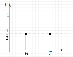
(1) discrete: a probability measure μ is discrete if all of its mass is at each individual point. The simplest example is a coin toss, whose graph is shown below:
(2) absolutely continuous: this property can refer to both random variable and measure and is defined differently. However, they are intrinsically connected, so both of them will be discussed here and it is important always to keep in mind the connection between a probability measure and a random variable.
a. Firstly we look at the case of measure. It is defined with regard to another measure, which serves as a reference. We say that ν is absolutely continuous with respect to μ, if ν(A) = 0 for any A ∈ 𝓑 such that μ(A) = 0. This relationship between ν and μ is usually denoted by ν ≪ μ. [2] We can also say that μ dominates ν. If it applies that both ν ≪ μ and μ ≪ ν, then we say that those two measures are equivalent, which is usually denoted as ν ~ μ. More intuitively, we can think of ν as a more “delicate” measure, if μ tells us that the measure of a set is zero, then ν will not output a larger result.
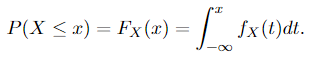
b. In the case of a random variable, a random variable X: Ω → ℝ is absolutely continuous if there exists an integrable non-negative function fₓ: ℝ → ℝ⁺ (this is the probability density function) such that for all x ∈ ℝ,
Sometimes we can also see that fₓ is integrable over all any Borel sets (elements in 𝓑), according to what we have discussed in section random variables, those two versions of the definition are the same.
Two questions arise: 1. what’s the relationship between “continuity” and “absolute continuity”? 2. What does continuity have to do with measure? (now we are only talking about random variables)
Firstly we will answer the second question: as discussed here, if P(X = x) = 0, for all the x ∈ ℝ, then X is a continuous variable. (Intuitively, when the random variable is continuous, it can take any value on the real line, and in this case, the measure gives us the “length of a point”). Now we look at the first question: From the definition of absolute continuity and we can derive
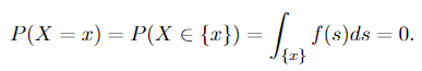
It is obvious why Equation 1.3 applies: the integration over a singleton set is zero. Since we have P(X = x) = 0 for all the x ∈ ℝ, as discussed above, X is continuous. Therefore, we have the statement:
Any absolutely continuous random variable is also continuous.
And the following fact builds the bridge between absolute continuity and measure:
A random variable is absolutely continuous if and only if every set of measure zero has zero probability.
(3) singularly continuous: here again, we have “singular continuous measure” and “singularly continuous distribution”, and again they are connected. And actually even closer to each other than in the previous case (continuity). We will look at the definitions of both of those concepts first and then give a concrete example. It is a topic, which is seldom included in the undergraduate study material. But after we get to know this, all the types of probability distributions are covered.
It is not necessary to go through the details of singular continuity if you just want to understand the Girsanov theorem, for which rather the “absolute continuity” is important. However, I believe it is helpful to learn the theory of probability, to understand all those types of distribution.
a. A singularly continuous distribution on ℝⁿ is a probability distribution concentrated on a set of Lebesgue measure zero, but the measure of every point in this set is also zero.
b. And a measure μ is singularly continuous with regard to measure λ if μ{x} = 0 for all x ∈ ℝ, but there is S ⊆ ℝ with λ(S) = 0 and μ(Sᶜ) = 0, which means μ(S) = 1. Another name, singular measure, can also be encountered and can appear to have slightly different definitions, but here for simplicity and clarity, we use the version in [1] and will avoid the term “singular measure”.
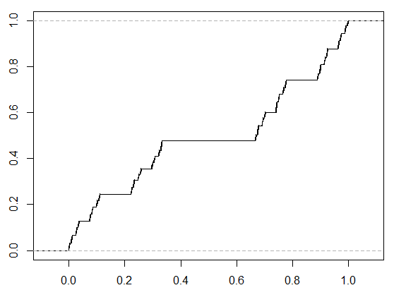
Some examples can be useful for understanding singular continuity. In the one-dimensional case (one random variable is involved), an example is Cantor’s function. Due to its shape, it is also referred to as the “devil’s staircase”. (see Figure 1.4) Such a cumulative distribution function (CDF) is continuous but has zero derivatives almost (we have seen this word before) everywhere. The bizarre thing is that it is not growing according to the derivative, but it is indeed increasing by construction.
Less pathological examples exist in higher dimensions (Think about this: we want to construct a set with Lebesgue measure zero, and in the set, every point will also have measure zero — naturally, this will be something like “the area of a line” or “the volume of a plane”, which cannot be found in one-dimensional space.), where the joint distribution of several random variables will be considered. Here we will show an example with two random variables taken from [4]:
There are two devices, which generate a random number from 0 to 1. However, one of them is broken and always gives 0. A statistician uses one of them each day, for two continuous days. He chooses randomly from those two devices (of course, it is possible that he uses the same device for both days). Let X represent the number acquired on the first day and Y denote the number acquired on the second day. What’s the joint distribution of X and Y?
We can easily see that this distribution is neither absolutely continuous nor discrete since the distribution of the output of the good device is uniform but that of the broken one is discrete. To analyze what it actually is, we will also talk about the decomposition of probability distribution via this example.
For a more intuitive understanding, here I offer a crappy scratch of the distribution function:
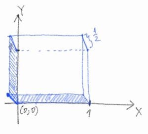
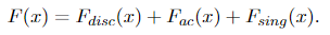
Note that f(0, 0) = 1/2, which means that half of the mass is concentrated on the point (0, 0). It corresponds to the event that on both days, the statistician gets output zero. And the other half of the mass is evenly spread on the one-by-one unit square (the volume is 1 × 1 × 1/2 = 1/2). We can also find the singular component in the CDF. Without loss of generality, we try to figure out the cumulative distribution of X first. According to Lebesgue’s decomposition theorem, any probability measure μ can be decomposed as

Since the CDF uniquely determines the distribution of a random variable (think of the definition), we can also decompose the CDF into the form given by Equation 1.6, namely
The CDF of X doesn’t have any singular part. And both discrete part and absolute continuous part can be easily determined:
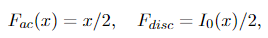
where Iᵣ(x) denotes the following function

Therefore, we have
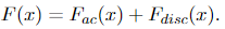
and according to the independent identical distribution (i.i.d.) assumption we talked about before, Y has the exact same CDF as X, given by Equation 1.10. Also, due to the i.i.d assumption, the CDF of X and Y is simply F(x, y) = F(x)F(y), which gives us
The joint CDF of X and Y have all three parts as expected. The singularly continuous part corresponds to the event that one of the devices is broken and another is good, which corresponds to the shaded area in the graph of the joint probability density function of X and Y given in Figure 1.5 — they have Lebesgue measure zero in three-dimensional space, and the measure defined on this space corresponding to the singular continuous part in Equation 1.11. But in this area, the measure of each point is zero.
Now we look back at the definition of singularly continuous measure, obviously, we can call the measure on the shaded area μ₁ (given that one of the devices is broken — a sub-sample space), and another μ₂ in the 3d space (the original sample space), we can see easily that μ₁ is singular with regard to μ₂.
Radon-Nikodym derivative
The Radon-Nikodym derivative is, in fact, a ratio of two measures, which has nothing to do with the “derivative” in real analysis, in the sense that the derivative in real analysis describes how fast a function changes, but the Radon-Nikodym derivative is nothing like this. However, they do have some similarities. We can see this from the following properties of the Radon-Nikodym derivative: Let ν be a σ-finite measure on a measure space (Ω, 𝓕) [7], (ν is σ-finite means that Ω is a countable union of sets with finite measures)
(1) if μ is a measure, μ ≪ ν and f ≥ 0 is a μ-integrable function, then
(2) If μᵢ, i= 1, 2 are measures and μᵢ ≪ ν, then μ₁ + μ₂ ≪ ν and
(3) (Chain rule) If 𝜏 is a measure, μ is a σ-finite measure, and 𝜏 ≪ μ ≪ ν, then
If μ and ν are equivalent, then
The Radon-Nikodym throrem
The Radon-Nikodym theorem shows a way to express one measure in terms of another measure via some linear operator. And in this case, the representation is via the integral operator (the integrator — this term is used here). The Radon-Nikodym theorem says
Given a measurable space (Ω, 𝓕), if a σ-finite measure ν on (Ω, 𝓕) is absolutely continuous with respect to a σ-finite measure μ on (Ω, 𝓕), then there is a non-negative measurable function f on Ω such that
for any measurable set E.
Why is this theorem important? One thing is that it can be used to show the existence of conditional expectation. Before we show the definition of the conditional expectation, we need to be aware of the fact that the conditional expectation of random variable X, given the σ-algebra 𝓕, denoted by E[X | 𝓕], is itself a (𝓕-measurable) random variable. The definition is given as follows:
We call a random variable Y to the conditional expectation of X, i.e. Y = E[X | 𝓕]. Two conditions need to be satisfied
(1) Y is 𝓕-measurable.
(2) For all A ∈ 𝓕, we have
1_A denotes the character (indicator) function. More intuitively, this means that given information 𝓕 (refer to this to see why it is called “information” and what it means), Y is the best prediction of X. And the following theorem, which can be proved using the Radon-Nikodym theorem, shows the existence and uniqueness of the conditional expectation:
Consider a probability space (Ω, 𝓕, P), a random variable X on it, and a sub-σ-algebra 𝓖 ⊆ 𝓕. If E[X] is well-defined, then there exists a 𝓖-measurable function E[X|𝓖] unique to P-null sets (the measure P gives zero on those sets), such that
The most important reason why we mention the Radon-Nikodym theorem in this is that it is closely related to the change of measure, which is fundamental in the Girsanov theorem. Now we present the following theorem:
If P and Q are equivalent probability measures, and X(t) is an 𝓕ₜ-adapted process, let dQ/dP be the Radon-Nikodym derivative and L(s) = Eₚ[dQ/dP|𝓕ₛ], then for s < t
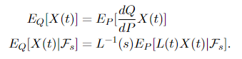
The second equality is quite technical to prove, so it’s not included here, but the first one is super easy to show using property (1) of the Radon-Nikodym derivative:
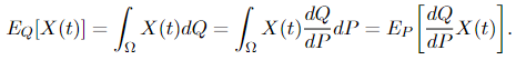
And the Radon-Nikodym theorem ensures that the Radon-Nikodym derivative dQ/dP exists, which is also known as the density of X.
Firstly, we briefly introduce what is Wiener measure because below we will be talking about Wiener processed and Wiener processes with drifts. The Wiener measure is the measure defined on Wiener space, which is the space C[0, 1] of continuous real-valued functions x on the interval [0, 1]. We can make a measurable space out of this, by equipping it with a σ-algebra and measure. And the Wiener measure is the unique measure on this space, which assigns a probability to every finite path. [5] Intuitively, the Wiener measure of a set is the probability that a Wiener process trajectory is a member of that set.
The Girsanov theorem states how a stochastic process change with the change of measure. To be more precise, it relates a Wiener measure P to a different measure Q on the space of continuous paths by giving an explicit formula for the likelihood ratios, which is the Radon-Nikodym derivative, between them. It also needs to apply that P and Q are equivalent, which is discussed in Section Continuity. And a bit more insight:
The Girsanov theorem says that a new process with a different drift can be constructed from a process with an equivalent measure — change in the drift of a stochastic process does not result in dramatic change in measure. And in fact, how the measure changes, can be calculated explictely.
A slightly different version of the Girsanov theorem states that a new representation can be found for a stochastic process, which has a different drift and measure.
There is also a converse version of the Girsanov theorem, which states that if we have a process X(t) with measure P, and another process Y(t) with measure Q, where Q ~ P. Then X(t) and Y(t) can be expressed in terms of each other with a drift change. We will introduce all three of these versions in this section. [6]
The Girsanov theorem I
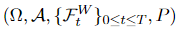
Let W(t) be a Wiener process on the filtered probability space
and let Y(t) ∈ ℝⁿ be an n-dimensional Itô process of the form

where T ≤ ∞ is a constant and W(t) is an n-dimensional Wiener process. Let measure
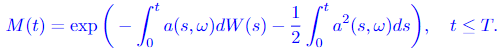
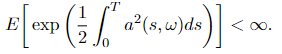
Assume that a(s, ω) satisfies Novikov’s condition, which is a sufficient condition for process M(t) to be a martingale:
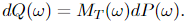
where E = Eₚ is the expectation with regard to P. Define the measure Q on the probability space of Y(t), (Ω, 𝓕_T), by
Then Y(t) is an n-dimensional Wiener process with regard to the probability measure Q, for t ≤ T.
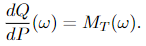
In this theorem, the Y(t) is the new process after a shift in the drift of a Wiener process. We can see that the a(t, ω) is the drift, which changes in time. The measure of Y(t) is given by transforming the original measure (the Wiener measure) P via the process Girsanov transformation given in Equation 3.2. And M(t), given by Equation 3.1, is the explicit formula of the change in measure between process W(t) and Y(t), which means it allows us to calculate the Radon-Nikodym derivative directly. We can see this trivially from Equation 3.2:
The Girsanov theorem II
The formulation of this version of the Girsanov theorem is very verbose because it is useful for the proof. But the proof is not included in this post since the purpose is to understand what is going on in (so many different formulations of) the Girsanov theorem, which is already tough enough. The second version shows how the measure changes when the drift of a process changes (or how can we find a different representation of a process, as we have mentioned before) and is given as follows:
Let Y(t) ∈ ℝⁿ be an Itô process of the form
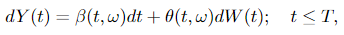
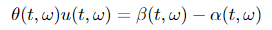
where W(t) ∈ ℝᵐ, β ∈ ℝⁿ and θ ∈ ℝⁿˣᵐ. Suppose there exists processes u(t, ω) and α(t, ω) such that
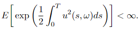
and assume that u(t, ω) satisfies Novikov’s condition
Let
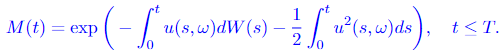
Measure P and Q are defined in the same way as in Girsanov theorem I, which means that E = Eₚ in Equation 3.3, and Equation 3.2 also applies. Then
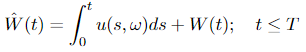
is a Wiener process with regard to measure Q and the process Y(t) has another representation in terms of W_hat(t)
In the Girsanov theorem II, we can see that the drift of Y(t) changes from β(t, ω) to α(t, ω). Also, as a side note, processes u(t, ω) and α(t, ω) should satisfy certain conditions, which are omitted here to make the big picture clear.
The converse of the Girsanov theorem
In logic, the converse of a statement p → q is q → p. In the Girasnov theorem, in simple words, p is the new measure, and q is the new process. Then the converse is formulated (with regard to Girsanov I, because it’s easier) as:
Let P be a Wiener measure of Wiener process W(t) and let Q~P be an equivalent measure on (Ω, 𝓐). Then there exists a stochastic process α(t, ω) ∈ ℝⁿ, 0 ≤ t ≤ T, adapted with regard to the history of W(t) (see Expression 3.0), such that

is a Wiener process on the probability space (Ω, 𝓐, Q). And the corresponding Radon-Nikodym is given by Equation 3.1. For convenient reference and the importance of this formula, we paste it here again

Summary
In this post, we started with the continuity of probability distribution — discrete, absolutely continuous, and singular continuous. Then the Radon-Nikodym derivative and theory are introduced, which is fundamental for the Girsanov theorem. In the last section, the Girsanov theorem is introduced. Two formulations of the Girsanov theorem are included, one is a change from the Wiener measure to another measure, and another one is switching between two different measures. At last, we show the converse of the Girsanov theorem. A very interesting and useful application of the Girsanov theorem is to make an asset price modeled by the Black-Scholes formula martingale. It is not included in this post since it is already lengthy enough. We will see it in an upcoming post about financial derivatives and the Black-Scholes formula.:)
Continuity of probability measure, Radon-Nikodym derivative, and Girsanov theorem

The Girsanov theorem and Radon-Nikodym theorem are frequently used in financial mathematics for the pricing of financial derivatives. And they are deeply related. The usage of those theorems can also be found in machine learning (very theoretical though). An example is given in [9], where Girsanov’s theory is applied in a new policy gradient algorithm for reinforcement learning.
However, those theorems are far from intuitive (even the notation). Therefore, this post attempts to offer a clear explanation to them, which is very difficult to find. To understand them properly, we need to understand different types of continuity of probability distribution first, that’s why this topic is also included and takes a large part of this post.
Also, note that this post is a continuation of this, things like filtration, martingale, Itô processes, etc. are already discussed there. So if something is not clear, you can refer to that post, or other two posts of mine about measure theory and theory of probability, or leave me a note.
Random variables and distribution
The random variable is a very basic concept in the theory of probability and it is also fundamental for understanding the stochastic processes. The random variable is slightly mentioned in my other posts about measure theory and probability, but here we will look at it more rigorously. Firstly, we show the formal definition of the random variable in the context of measure theory:
Given a probability triple (Ω, 𝓕, P), a random variable is a function X from Ω to the real numbers ℝ, such that
We can see that ω is the image of X and Condition 1.1 is the same as saying X⁻¹((-∞, x]) ∈ 𝓕. Also, we know that if set A ={(-∞, x]; x ∈ ℝ}, then σ(A) = 𝓑, where 𝓑 is the Borel σ-algebra. (This can be proved easily by proving that σ(A) contains all the intervals using the properties of σ-algebra.) Therefore, Condition 1.1 is also the same as X⁻¹(B) ∈ 𝓕, for all B ∈ 𝓑. [1]
The distribution of a random variable on a probability triple (Ω, 𝓕, P) is P (recall that it is a function defined on ), the measure of the probability space. The distribution is defined by (or in other words, the probability is defined in terms of a random variable by)
Note that sometimes you can also see the term “probability law” or “law” of a random variable, but they are the same thing.
Continuity
We already know that a random variable or a distribution can be discrete, continuous, or a combination of both. But there is still something missing, and in this section, we will review what we already knew and fill the gap.
(1) discrete: a probability measure μ is discrete if all of its mass is at each individual point. The simplest example is a coin toss, whose graph is shown below:
(2) absolutely continuous: this property can refer to both random variable and measure and is defined differently. However, they are intrinsically connected, so both of them will be discussed here and it is important always to keep in mind the connection between a probability measure and a random variable.
a. Firstly we look at the case of measure. It is defined with regard to another measure, which serves as a reference. We say that ν is absolutely continuous with respect to μ, if ν(A) = 0 for any A ∈ 𝓑 such that μ(A) = 0. This relationship between ν and μ is usually denoted by ν ≪ μ. [2] We can also say that μ dominates ν. If it applies that both ν ≪ μ and μ ≪ ν, then we say that those two measures are equivalent, which is usually denoted as ν ~ μ. More intuitively, we can think of ν as a more “delicate” measure, if μ tells us that the measure of a set is zero, then ν will not output a larger result.
b. In the case of a random variable, a random variable X: Ω → ℝ is absolutely continuous if there exists an integrable non-negative function fₓ: ℝ → ℝ⁺ (this is the probability density function) such that for all x ∈ ℝ,
Sometimes we can also see that fₓ is integrable over all any Borel sets (elements in 𝓑), according to what we have discussed in section random variables, those two versions of the definition are the same.
Two questions arise: 1. what’s the relationship between “continuity” and “absolute continuity”? 2. What does continuity have to do with measure? (now we are only talking about random variables)
Firstly we will answer the second question: as discussed here, if P(X = x) = 0, for all the x ∈ ℝ, then X is a continuous variable. (Intuitively, when the random variable is continuous, it can take any value on the real line, and in this case, the measure gives us the “length of a point”). Now we look at the first question: From the definition of absolute continuity and we can derive
It is obvious why Equation 1.3 applies: the integration over a singleton set is zero. Since we have P(X = x) = 0 for all the x ∈ ℝ, as discussed above, X is continuous. Therefore, we have the statement:
Any absolutely continuous random variable is also continuous.
And the following fact builds the bridge between absolute continuity and measure:
A random variable is absolutely continuous if and only if every set of measure zero has zero probability.
(3) singularly continuous: here again, we have “singular continuous measure” and “singularly continuous distribution”, and again they are connected. And actually even closer to each other than in the previous case (continuity). We will look at the definitions of both of those concepts first and then give a concrete example. It is a topic, which is seldom included in the undergraduate study material. But after we get to know this, all the types of probability distributions are covered.
It is not necessary to go through the details of singular continuity if you just want to understand the Girsanov theorem, for which rather the “absolute continuity” is important. However, I believe it is helpful to learn the theory of probability, to understand all those types of distribution.
a. A singularly continuous distribution on ℝⁿ is a probability distribution concentrated on a set of Lebesgue measure zero, but the measure of every point in this set is also zero.
b. And a measure μ is singularly continuous with regard to measure λ if μ{x} = 0 for all x ∈ ℝ, but there is S ⊆ ℝ with λ(S) = 0 and μ(Sᶜ) = 0, which means μ(S) = 1. Another name, singular measure, can also be encountered and can appear to have slightly different definitions, but here for simplicity and clarity, we use the version in [1] and will avoid the term “singular measure”.
Some examples can be useful for understanding singular continuity. In the one-dimensional case (one random variable is involved), an example is Cantor’s function. Due to its shape, it is also referred to as the “devil’s staircase”. (see Figure 1.4) Such a cumulative distribution function (CDF) is continuous but has zero derivatives almost (we have seen this word before) everywhere. The bizarre thing is that it is not growing according to the derivative, but it is indeed increasing by construction.
Less pathological examples exist in higher dimensions (Think about this: we want to construct a set with Lebesgue measure zero, and in the set, every point will also have measure zero — naturally, this will be something like “the area of a line” or “the volume of a plane”, which cannot be found in one-dimensional space.), where the joint distribution of several random variables will be considered. Here we will show an example with two random variables taken from [4]:
There are two devices, which generate a random number from 0 to 1. However, one of them is broken and always gives 0. A statistician uses one of them each day, for two continuous days. He chooses randomly from those two devices (of course, it is possible that he uses the same device for both days). Let X represent the number acquired on the first day and Y denote the number acquired on the second day. What’s the joint distribution of X and Y?
We can easily see that this distribution is neither absolutely continuous nor discrete since the distribution of the output of the good device is uniform but that of the broken one is discrete. To analyze what it actually is, we will also talk about the decomposition of probability distribution via this example.
For a more intuitive understanding, here I offer a crappy scratch of the distribution function:
Note that f(0, 0) = 1/2, which means that half of the mass is concentrated on the point (0, 0). It corresponds to the event that on both days, the statistician gets output zero. And the other half of the mass is evenly spread on the one-by-one unit square (the volume is 1 × 1 × 1/2 = 1/2). We can also find the singular component in the CDF. Without loss of generality, we try to figure out the cumulative distribution of X first. According to Lebesgue’s decomposition theorem, any probability measure μ can be decomposed as
Since the CDF uniquely determines the distribution of a random variable (think of the definition), we can also decompose the CDF into the form given by Equation 1.6, namely
The CDF of X doesn’t have any singular part. And both discrete part and absolute continuous part can be easily determined:
where Iᵣ(x) denotes the following function
Therefore, we have
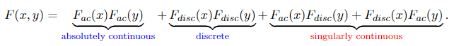
and according to the independent identical distribution (i.i.d.) assumption we talked about before, Y has the exact same CDF as X, given by Equation 1.10. Also, due to the i.i.d assumption, the CDF of X and Y is simply F(x, y) = F(x)F(y), which gives us
The joint CDF of X and Y have all three parts as expected. The singularly continuous part corresponds to the event that one of the devices is broken and another is good, which corresponds to the shaded area in the graph of the joint probability density function of X and Y given in Figure 1.5 — they have Lebesgue measure zero in three-dimensional space, and the measure defined on this space corresponding to the singular continuous part in Equation 1.11. But in this area, the measure of each point is zero.
Now we look back at the definition of singularly continuous measure, obviously, we can call the measure on the shaded area μ₁ (given that one of the devices is broken — a sub-sample space), and another μ₂ in the 3d space (the original sample space), we can see easily that μ₁ is singular with regard to μ₂.
Radon-Nikodym derivative
The Radon-Nikodym derivative is, in fact, a ratio of two measures, which has nothing to do with the “derivative” in real analysis, in the sense that the derivative in real analysis describes how fast a function changes, but the Radon-Nikodym derivative is nothing like this. However, they do have some similarities. We can see this from the following properties of the Radon-Nikodym derivative: Let ν be a σ-finite measure on a measure space (Ω, 𝓕) [7], (ν is σ-finite means that Ω is a countable union of sets with finite measures)
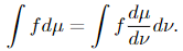
(1) if μ is a measure, μ ≪ ν and f ≥ 0 is a μ-integrable function, then
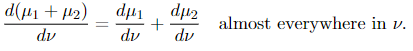
(2) If μᵢ, i= 1, 2 are measures and μᵢ ≪ ν, then μ₁ + μ₂ ≪ ν and
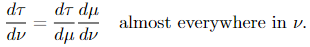
(3) (Chain rule) If 𝜏 is a measure, μ is a σ-finite measure, and 𝜏 ≪ μ ≪ ν, then
If μ and ν are equivalent, then
The Radon-Nikodym throrem
The Radon-Nikodym theorem shows a way to express one measure in terms of another measure via some linear operator. And in this case, the representation is via the integral operator (the integrator — this term is used here). The Radon-Nikodym theorem says
Given a measurable space (Ω, 𝓕), if a σ-finite measure ν on (Ω, 𝓕) is absolutely continuous with respect to a σ-finite measure μ on (Ω, 𝓕), then there is a non-negative measurable function f on Ω such that
for any measurable set E.
Why is this theorem important? One thing is that it can be used to show the existence of conditional expectation. Before we show the definition of the conditional expectation, we need to be aware of the fact that the conditional expectation of random variable X, given the σ-algebra 𝓕, denoted by E[X | 𝓕], is itself a (𝓕-measurable) random variable. The definition is given as follows:
We call a random variable Y to the conditional expectation of X, i.e. Y = E[X | 𝓕]. Two conditions need to be satisfied
(1) Y is 𝓕-measurable.
(2) For all A ∈ 𝓕, we have
1_A denotes the character (indicator) function. More intuitively, this means that given information 𝓕 (refer to this to see why it is called “information” and what it means), Y is the best prediction of X. And the following theorem, which can be proved using the Radon-Nikodym theorem, shows the existence and uniqueness of the conditional expectation:
Consider a probability space (Ω, 𝓕, P), a random variable X on it, and a sub-σ-algebra 𝓖 ⊆ 𝓕. If E[X] is well-defined, then there exists a 𝓖-measurable function E[X|𝓖] unique to P-null sets (the measure P gives zero on those sets), such that
The most important reason why we mention the Radon-Nikodym theorem in this is that it is closely related to the change of measure, which is fundamental in the Girsanov theorem. Now we present the following theorem:
If P and Q are equivalent probability measures, and X(t) is an 𝓕ₜ-adapted process, let dQ/dP be the Radon-Nikodym derivative and L(s) = Eₚ[dQ/dP|𝓕ₛ], then for s < t
The second equality is quite technical to prove, so it’s not included here, but the first one is super easy to show using property (1) of the Radon-Nikodym derivative:
And the Radon-Nikodym theorem ensures that the Radon-Nikodym derivative dQ/dP exists, which is also known as the density of X.
Firstly, we briefly introduce what is Wiener measure because below we will be talking about Wiener processed and Wiener processes with drifts. The Wiener measure is the measure defined on Wiener space, which is the space C[0, 1] of continuous real-valued functions x on the interval [0, 1]. We can make a measurable space out of this, by equipping it with a σ-algebra and measure. And the Wiener measure is the unique measure on this space, which assigns a probability to every finite path. [5] Intuitively, the Wiener measure of a set is the probability that a Wiener process trajectory is a member of that set.
The Girsanov theorem states how a stochastic process change with the change of measure. To be more precise, it relates a Wiener measure P to a different measure Q on the space of continuous paths by giving an explicit formula for the likelihood ratios, which is the Radon-Nikodym derivative, between them. It also needs to apply that P and Q are equivalent, which is discussed in Section Continuity. And a bit more insight:
The Girsanov theorem says that a new process with a different drift can be constructed from a process with an equivalent measure — change in the drift of a stochastic process does not result in dramatic change in measure. And in fact, how the measure changes, can be calculated explictely.
A slightly different version of the Girsanov theorem states that a new representation can be found for a stochastic process, which has a different drift and measure.
There is also a converse version of the Girsanov theorem, which states that if we have a process X(t) with measure P, and another process Y(t) with measure Q, where Q ~ P. Then X(t) and Y(t) can be expressed in terms of each other with a drift change. We will introduce all three of these versions in this section. [6]
The Girsanov theorem I
Let W(t) be a Wiener process on the filtered probability space
and let Y(t) ∈ ℝⁿ be an n-dimensional Itô process of the form
where T ≤ ∞ is a constant and W(t) is an n-dimensional Wiener process. Let measure
Assume that a(s, ω) satisfies Novikov’s condition, which is a sufficient condition for process M(t) to be a martingale:
where E = Eₚ is the expectation with regard to P. Define the measure Q on the probability space of Y(t), (Ω, 𝓕_T), by
Then Y(t) is an n-dimensional Wiener process with regard to the probability measure Q, for t ≤ T.
In this theorem, the Y(t) is the new process after a shift in the drift of a Wiener process. We can see that the a(t, ω) is the drift, which changes in time. The measure of Y(t) is given by transforming the original measure (the Wiener measure) P via the process Girsanov transformation given in Equation 3.2. And M(t), given by Equation 3.1, is the explicit formula of the change in measure between process W(t) and Y(t), which means it allows us to calculate the Radon-Nikodym derivative directly. We can see this trivially from Equation 3.2:
The Girsanov theorem II
The formulation of this version of the Girsanov theorem is very verbose because it is useful for the proof. But the proof is not included in this post since the purpose is to understand what is going on in (so many different formulations of) the Girsanov theorem, which is already tough enough. The second version shows how the measure changes when the drift of a process changes (or how can we find a different representation of a process, as we have mentioned before) and is given as follows:
Let Y(t) ∈ ℝⁿ be an Itô process of the form
where W(t) ∈ ℝᵐ, β ∈ ℝⁿ and θ ∈ ℝⁿˣᵐ. Suppose there exists processes u(t, ω) and α(t, ω) such that
and assume that u(t, ω) satisfies Novikov’s condition
Let
Measure P and Q are defined in the same way as in Girsanov theorem I, which means that E = Eₚ in Equation 3.3, and Equation 3.2 also applies. Then
is a Wiener process with regard to measure Q and the process Y(t) has another representation in terms of W_hat(t)
In the Girsanov theorem II, we can see that the drift of Y(t) changes from β(t, ω) to α(t, ω). Also, as a side note, processes u(t, ω) and α(t, ω) should satisfy certain conditions, which are omitted here to make the big picture clear.
The converse of the Girsanov theorem
In logic, the converse of a statement p → q is q → p. In the Girasnov theorem, in simple words, p is the new measure, and q is the new process. Then the converse is formulated (with regard to Girsanov I, because it’s easier) as:
Let P be a Wiener measure of Wiener process W(t) and let Q~P be an equivalent measure on (Ω, 𝓐). Then there exists a stochastic process α(t, ω) ∈ ℝⁿ, 0 ≤ t ≤ T, adapted with regard to the history of W(t) (see Expression 3.0), such that
is a Wiener process on the probability space (Ω, 𝓐, Q). And the corresponding Radon-Nikodym is given by Equation 3.1. For convenient reference and the importance of this formula, we paste it here again
Summary
In this post, we started with the continuity of probability distribution — discrete, absolutely continuous, and singular continuous. Then the Radon-Nikodym derivative and theory are introduced, which is fundamental for the Girsanov theorem. In the last section, the Girsanov theorem is introduced. Two formulations of the Girsanov theorem are included, one is a change from the Wiener measure to another measure, and another one is switching between two different measures. At last, we show the converse of the Girsanov theorem. A very interesting and useful application of the Girsanov theorem is to make an asset price modeled by the Black-Scholes formula martingale. It is not included in this post since it is already lengthy enough. We will see it in an upcoming post about financial derivatives and the Black-Scholes formula.:)
Denial of responsibility! Techno Blender is an automatic aggregator of the all world’s media. In each content, the hyperlink to the primary source is specified. All trademarks belong to their rightful owners, all materials to their authors. If you are the owner of the content and do not want us to publish your materials, please contact us by email – [email protected]. The content will be deleted within 24 hours.