Backpropagation — Chain Rule and PyTorch in Action | by Robert Kwiatkowski | Jul, 2022

A simple guide from theory to implementation in Pytorch.

The modern businesses rely more and more on the advances in the innovative fields like Artificial Intelligence to deliver the best product and services to its customers. Many of production AI systems is based on various Neural Networks trained often using a tremendous amount of data. For development teams one of the biggest challenges is how to train their models in a constrained time frame. There are various techniques and algorithms to do it but the most popular are these using some kind of gradient descent method.

The training of Neural Networks (NN) based on gradient-based optimization algorithms is organized in two major steps:

1. Forward Propagation — here we calculate the output of the NN given inputs
2. Backward Propagation — here we calculate the gradients of the output with regards to inputs to update the weights

The first step is usually straightforward to understand and to calculate. The general idea behind the second step is also clear — we need gradients to know the direction to make steps in gradient descent optimization algorithm. If you are not familiar with this method you can check my other article (Gradient Descent Algorithm — a deep dive).

Although the backpropagation is not a new idea (developed in 1970s), answering the question “how” these gradients are calculated gives some people a hard time. One has to reach for some calculus, especially partial derivatives and the chain rule, to fully understand back-propagation working principles.

Originally backpropagation was developed to differentiate complex nested functions. However, it became highly popular thanks to the machine learning community and is now the cornerstone of Neural Networks.

In this article we’ll go to the roots and solve an exemplary problem step-by-step by hand, then we’ll implement it in python using PyTorch, and finally we’re going to compare both results to make sure everything works fine.

1. Computational Graph

Let’s assume we want to perform the following set of operations to get our result r:

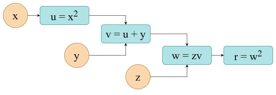
If you substitute all individual node-equations into the final one you’ll find that we’re solving the following equation. Being more specific we want to calculate its value and its partial derivatives. So in this use case it is a pure mathematical task.

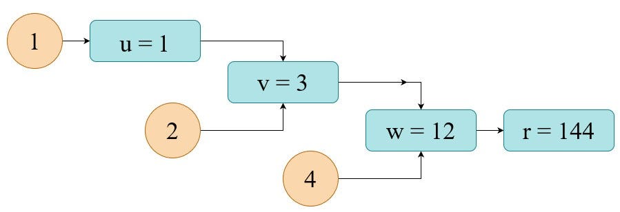
2. Forward Pass

To make this concept more tangible let’s take some numbers for our calculation. For example:

Here we simply substitute our inputs into equations. The results of individual node-steps are shown below. The final output is r=144.

3. Backward Pass

Now it’s time to perform a backpropagation, known also under a more fancy name “backward propagation of errors” or even “reverse mode of automatic differentiation”.

To calculate gradients with regards to each of 3 variables we have to calculate partial derivatives at each node in the graph (local gradients). Below I show you how to do it for the two last nodes/steps (I’ll leave the rest as an exercise).

After completing the calculations of local gradients a computation graph for the back-propagation is like below.

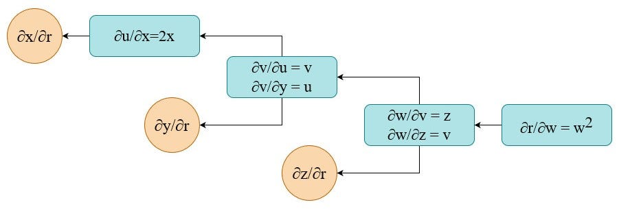
Now, to calculate the final gradients (in orange circles) we have to use the chain rule. In practice this means we have to multiply all partial derivatives along the path from the output to the variable of interest:

Now we can use these gradient for whatever we want — e.g. optimization with a gradient descent (SGD, Adam, etc.).

4. Implementation in PyTorch

There are numerous Neural Network frameworks in various languages where you can implement such computations and make a computer to calculate gradients for you. Below, I’ll demonstrate how to use the python PyTorch library to solve our exemplary task.

The output of this code is:

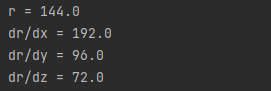
Results from PyTorch are identical to the ones we calculated by hand.

Couple of notes:

• In PyTorch everything is a tensor — even if it contains only a single value
• In PyTorch when you specify a variable which is a subject of gradient-based optimization you have to specify argument requires_grad = True. Otherwise, it will be treated as fixed input
• With this implementation, all back-propagation calculations are simply performed by using method r.backward()

5. Summary

In this article we used backpropagation to solve a specific mathematical problem — to calculate partial derivatives of a complex function. However, when you define the architecture of a Neural Network you are de facto creating a calculation graph and all the principles seen here still hold.

In NNs the final equation is then a loss function of your choice, e.g. MSE, MAE and the node equations are mostly weights/arguments multiplications followed by various activation functions (ReLu, tanh, softmax, etc.)

Hopefully, now you feel more confident in answering the question of how the back-propagation works, why do we need it and how to implement it in PyTorch.

Happy coding!

A simple guide from theory to implementation in Pytorch.

The modern businesses rely more and more on the advances in the innovative fields like Artificial Intelligence to deliver the best product and services to its customers. Many of production AI systems is based on various Neural Networks trained often using a tremendous amount of data. For development teams one of the biggest challenges is how to train their models in a constrained time frame. There are various techniques and algorithms to do it but the most popular are these using some kind of gradient descent method.

The training of Neural Networks (NN) based on gradient-based optimization algorithms is organized in two major steps:

1. Forward Propagation — here we calculate the output of the NN given inputs
2. Backward Propagation — here we calculate the gradients of the output with regards to inputs to update the weights

The first step is usually straightforward to understand and to calculate. The general idea behind the second step is also clear — we need gradients to know the direction to make steps in gradient descent optimization algorithm. If you are not familiar with this method you can check my other article (Gradient Descent Algorithm — a deep dive).

Although the backpropagation is not a new idea (developed in 1970s), answering the question “how” these gradients are calculated gives some people a hard time. One has to reach for some calculus, especially partial derivatives and the chain rule, to fully understand back-propagation working principles.

Originally backpropagation was developed to differentiate complex nested functions. However, it became highly popular thanks to the machine learning community and is now the cornerstone of Neural Networks.

In this article we’ll go to the roots and solve an exemplary problem step-by-step by hand, then we’ll implement it in python using PyTorch, and finally we’re going to compare both results to make sure everything works fine.

1. Computational Graph

Let’s assume we want to perform the following set of operations to get our result r:

If you substitute all individual node-equations into the final one you’ll find that we’re solving the following equation. Being more specific we want to calculate its value and its partial derivatives. So in this use case it is a pure mathematical task.

2. Forward Pass

To make this concept more tangible let’s take some numbers for our calculation. For example:

Here we simply substitute our inputs into equations. The results of individual node-steps are shown below. The final output is r=144.

3. Backward Pass

Now it’s time to perform a backpropagation, known also under a more fancy name “backward propagation of errors” or even “reverse mode of automatic differentiation”.

To calculate gradients with regards to each of 3 variables we have to calculate partial derivatives at each node in the graph (local gradients). Below I show you how to do it for the two last nodes/steps (I’ll leave the rest as an exercise).

After completing the calculations of local gradients a computation graph for the back-propagation is like below.

Now, to calculate the final gradients (in orange circles) we have to use the chain rule. In practice this means we have to multiply all partial derivatives along the path from the output to the variable of interest:

Now we can use these gradient for whatever we want — e.g. optimization with a gradient descent (SGD, Adam, etc.).

4. Implementation in PyTorch

There are numerous Neural Network frameworks in various languages where you can implement such computations and make a computer to calculate gradients for you. Below, I’ll demonstrate how to use the python PyTorch library to solve our exemplary task.

The output of this code is:

Results from PyTorch are identical to the ones we calculated by hand.

Couple of notes:

• In PyTorch everything is a tensor — even if it contains only a single value
• In PyTorch when you specify a variable which is a subject of gradient-based optimization you have to specify argument requires_grad = True. Otherwise, it will be treated as fixed input
• With this implementation, all back-propagation calculations are simply performed by using method r.backward()

5. Summary

In this article we used backpropagation to solve a specific mathematical problem — to calculate partial derivatives of a complex function. However, when you define the architecture of a Neural Network you are de facto creating a calculation graph and all the principles seen here still hold.

In NNs the final equation is then a loss function of your choice, e.g. MSE, MAE and the node equations are mostly weights/arguments multiplications followed by various activation functions (ReLu, tanh, softmax, etc.)

Hopefully, now you feel more confident in answering the question of how the back-propagation works, why do we need it and how to implement it in PyTorch.

Happy coding!