
Bounded Kernel Density Estimation
Learn how Kernel Density Estimation works and how you can adjust it to better handle bounded data, like age, height, or price
Histograms are widely used and easily grasped, but when it comes to estimating continuous densities, people often resort to treating it as a mysterious black box. However, understanding this concept is just as straightforward and becomes crucial, especially when dealing with bounded data like age, height, or price, where available libraries may not handle it automatically.
1. Kernel Density Estimation
Histogram
A histogram involves partitioning the data range into bins or sub-intervals and counting the number of samples that fall within each bin. It thus approximates the continuous density function with a piecewise constant function.
- Large bin size: It helps capturing the low-frequency outline of the density function, by gathering neighboring samples to avoid empty bins. However, it looses the continuity property because there could be a significant gap between the count of adjacent bins.
- Small bin size: It helps capturing details at higher frequencies. However, if the number of samples is too small, we’ll end up with lots of empty bins at places where the true density isn’t.

Kernel Density Estimation (KDE)
An intuitive idea is to assume that the density function from which the samples are drawn is smooth, and leverage it to fill-in the gaps of our high frequency histogram.
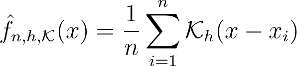
This is precisely what the Kernel Density Estimation (KDE) does. It estimates the global density as the average of local density kernels K centered around each sample. A Kernel is a non-negative function integrating to 1, e.g uniform, triangular, normal… Just like adjusting the bin size in a histogram, we introduce a bandwidth parameter h that modulates the deviation of the kernel around each sample point. It thus controls the smoothness of the resulting density estimate.
Bandwith Selection
Finding the right balance between under- and over-smoothing isn’t straightforward. A popular and easy-to-compute heuristic is the Silverman’s rule of thumb, which is optimal when the underlying density being estimated is Gaussian.
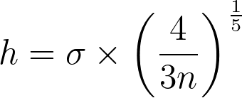
Keep in mind that it may not always yield optimal results across all data distributions. I won’t discuss them in this article, but there are other alternatives and improvements available.
The image below depicts a Gaussian distribution being estimated by a gaussian KDE at different bandwidth values. As we can see, Silverman’s rule of thumb is well-suited, but higher bandwidths cause over-smoothing, while lower ones introduce high-frequency oscillations around the true density.
Examples
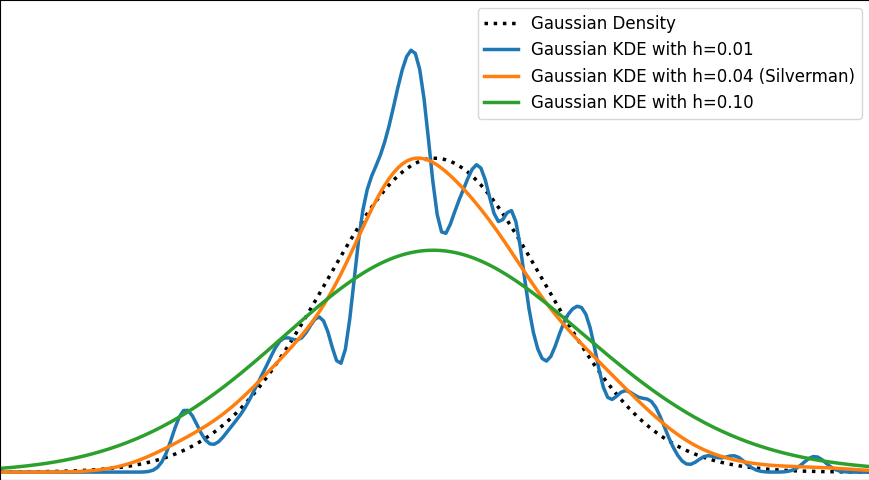
The video below illustrates the convergence of a Kernel Density Estimation with a Gaussian kernel across 4 standard density distributions as the number of provided samples increases.
Although it’s not optimal, I’ve chosen to keep a small constant bandwidth h over the video to better illustrate the process of kernel averaging, and to prevent excessive smoothing when the sample size is very small.
Implementation of Gaussian Kernel Density Estimation
Great python libraries like scipy and scikit-learn provide public implementations for Kernel Density Estimation:
- scipy.stats.gaussian_kde
- sklearn.neighbors.KernelDensity
However, it’s valuable to note that a basic equivalent can be built in just three lines using numpy. We need the samples x_data drawn from the distribution to estimate and the points x_prediction at which we want to evaluate the density estimate. Then, using array broadcasting we can evaluate a local gaussian kernel around each input sample and average them into the final density estimate.
N.B. This version is fast because it’s vectorized. However it involves creating a large 2D temporary array of shape (len(x_data), len(x_prediction)) to store all the kernel evaluations. To have a lower memory footprint, we could re-write it using numba or cython (to avoid the computational burden of Python for loops) to aggregate kernel evaluations on-the-fly in a running sum for each output prediction.
https://medium.com/media/075f9f863177fe88993e0edee2cfba06/href
2. Handle boundaries
Bounded Distributions
Real-life data is often bounded by a given domain. For example, attributes such as age, weight, or duration are always non-negative values. In such scenarios, a standard smooth KDE may fail to accurately capture the true shape of the distribution, especially if there’s a density discontinuity at the boundary.
In 1D, with the exception of some exotic cases, bounded distributions typically have either one-sided (e.g. positive values) or two-sided (e.g. uniform interval) bounded domains.
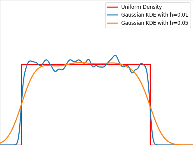
As illustrated in the graph below, kernels are bad at estimating the edges of the uniform distribution and leak outside the bounded domain.
No Clean Public Solution in Python
Unfortunately, popular public Python libraries like scipy and scikit-learn do not currently address this issue. There are existing GitHub issues and pull requests discussing this topic, but regrettably, they have remained unresolved for quite some time.
- Feature Request: KDE for Bounded Data (GitHub Issue scikit-learn — 2017)
- ENH: improve stats.kde density estimation near boundaries (GitHub Pull Request scipy — 2016)
In R, kde.boundary allows Kernel density estimate for bounded data.
There are various ways to take into account the bounded nature of the distribution. Let’s describe the most popular ones: Reflection, Weighting and Transformation.
Warning:
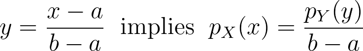
For the sake of readability, we will focus on the unit bounded domain, i.e. [0,1]. Please remember to standardize the data and scale the density appropriately in the general case [a,b].
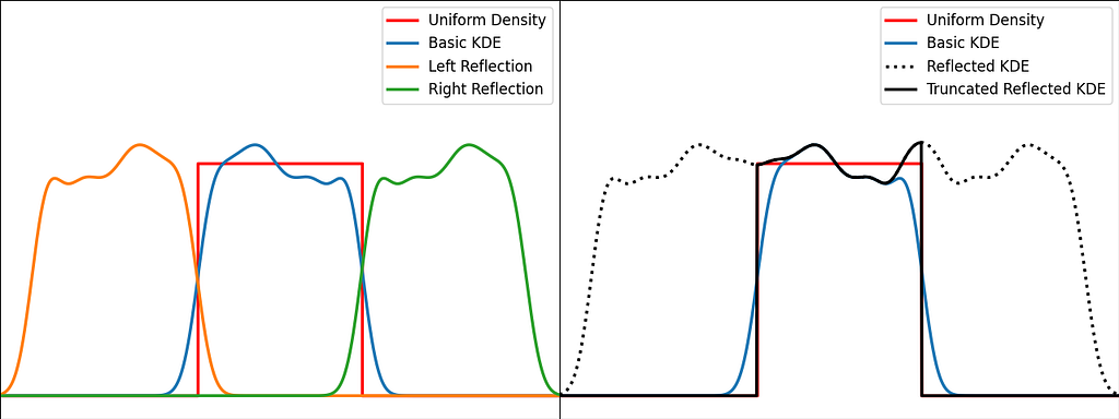
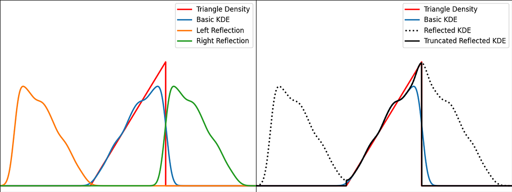
Solution: Reflection
The trick is to augment the set of samples by reflecting them across the left and right boundaries. This is equivalent to reflecting the tails of the local kernels to keep them in the bounded domain. It works best when the density derivative is zero at the boundary.
The reflection technique also implies processing three times more sample points.
The graphs below illustrate the reflection trick for three standard distributions: uniform, right triangle and inverse square root. It does a pretty good job at reducing the bias at the boundaries, even for the singularity of the inverse square root distribution.

https://medium.com/media/a2eb5b5f06fd73d71126fd0f9426fbad/href
N.B. The signature of basic_kde has been slightly updated to allow to optionally provide your own bandwidth parameter instead of using the Silverman’s rule of thumb.
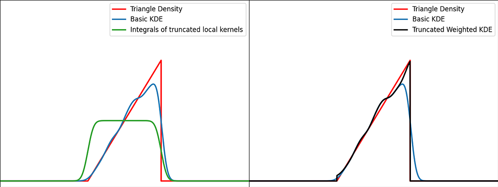
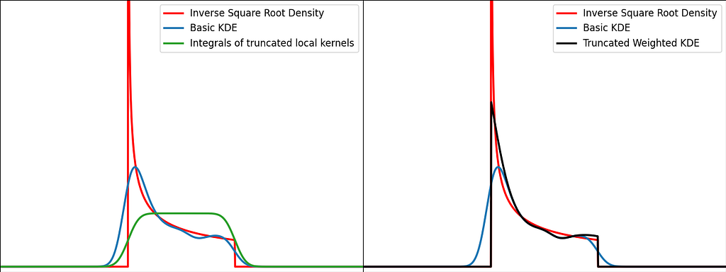
Solution: Weighting
The reflection trick presented above takes the leaking tails of the local kernel and add them back to the bounded domain, so that the information isn’t lost. However, we could also compute how much of our local kernel has been lost outside the bounded domain and leverage it to correct the bias.
For a very large number of samples, the KDE converges to the convolution between the kernel and the true density, truncated by the bounded domain.

If x is at a boundary, then only half of the kernel area will actually be used. Intuitively, we’d like to normalize the convolution kernel to make it integrate to 1 over the bounded domain. The integral will be close to 1 at the center of the bounded interval and will fall off to 0.5 near the borders. This accounts for the lack of neighboring kernels at the boundaries.
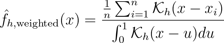
Similarly to the reflection technique, the graphs below illustrate the weighting trick for three standard distributions: uniform, right triangle and inverse square root. It performs very similarly to the reflection method.
From a computational perspective, it doesn’t require to process 3 times more samples, but it needs to evaluate the normal Cumulative Density Function at the prediction points.

https://medium.com/media/1153893cb61b3f1cc77136a51684cf69/href
Transformation
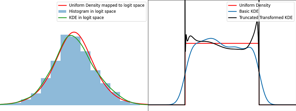
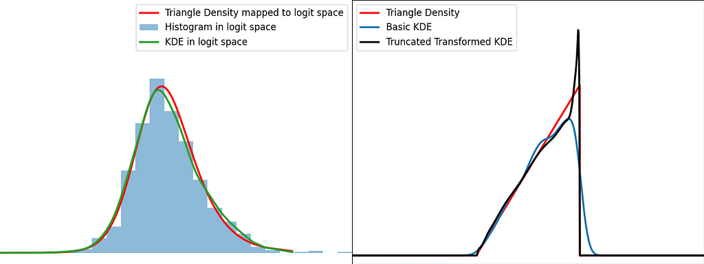
The transformation trick maps the bounded data to an unbounded space, where the KDE can be safely applied. This results in using a different kernel function for each input sample.
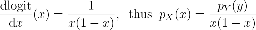
The logit function leverages the logarithm to map the unit interval [0,1] to the entire real axis.

When applying a transform f onto a random variable X, the resulting density can be obtained by dividing by the absolute value of the derivative of f.
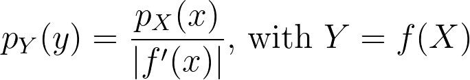
We can now apply it for the special case of the logit transform to retrieve the density distribution from the one estimated in the logit space.
Similarly to the reflection and weighting techniques, the graphs below illustrate the weighting trick for three standard distributions: uniform, right triangle and inverse square root. It performs quite poorly by creating large oscillations at the boundaries. However, it handles extremely well the singularity of the inverse square root.

https://medium.com/media/219eb8103b5c9060e66713f82b9eb184/href

Conclusion
Histograms and KDE
In Kernel Density Estimation, each sample is assigned its own local kernel density centered around it, and then we average all these densities to obtain the global density. The bandwidth parameter defines how far the influence of each kernel extends. Intuitively, we should decrease the bandwidth as the number of samples increases, to prevent excessive smoothing.
Histograms can be seen as a simplified version of KDE. Indeed, the bins implicitly define a finite set of possible rectangular kernels, and each sample is assigned to the closest one. Finally, the average of all these densities result in a piecewise-constant estimate of the global density.
Which method is the best ?
Reflection, weighting and transform are efficient basic methods to handle bounded data during KDE. However, bear in mind that there isn’t a one-size-fits-all solution; it heavily depends on the shape of your data.
The transform method handles pretty well the singularities, as we’ve seen with the inverse square root distribution. As for reflection and weighting, they are generally more suitable for a broader range of scenarios.
Reflection introduces complexity during training, whereas weighting adds complexity during inference.
From [0,1] to [a,b], [a, +∞[ and ]-∞,b]
Code presented above has been written for data bounded in the unit interval. Don’t forget to scale the density, when applying the affine transformation to normalize your data.
It can also easily be adjusted for a one-sided bounded domain, by reflecting only on one side, integrating the kernel to infinity on one side or using the logarithm instead of logit.
I hope you enjoyed reading this article and that it gave you more insights on how Kernel Density Estimation works and how to handle bounded domains!
Bounded Kernel Density Estimation was originally published in Towards Data Science on Medium, where people are continuing the conversation by highlighting and responding to this story.
Learn how Kernel Density Estimation works and how you can adjust it to better handle bounded data, like age, height, or price

Histograms are widely used and easily grasped, but when it comes to estimating continuous densities, people often resort to treating it as a mysterious black box. However, understanding this concept is just as straightforward and becomes crucial, especially when dealing with bounded data like age, height, or price, where available libraries may not handle it automatically.
1. Kernel Density Estimation
Histogram
A histogram involves partitioning the data range into bins or sub-intervals and counting the number of samples that fall within each bin. It thus approximates the continuous density function with a piecewise constant function.
- Large bin size: It helps capturing the low-frequency outline of the density function, by gathering neighboring samples to avoid empty bins. However, it looses the continuity property because there could be a significant gap between the count of adjacent bins.
- Small bin size: It helps capturing details at higher frequencies. However, if the number of samples is too small, we’ll end up with lots of empty bins at places where the true density isn’t.
Kernel Density Estimation (KDE)
An intuitive idea is to assume that the density function from which the samples are drawn is smooth, and leverage it to fill-in the gaps of our high frequency histogram.
This is precisely what the Kernel Density Estimation (KDE) does. It estimates the global density as the average of local density kernels K centered around each sample. A Kernel is a non-negative function integrating to 1, e.g uniform, triangular, normal… Just like adjusting the bin size in a histogram, we introduce a bandwidth parameter h that modulates the deviation of the kernel around each sample point. It thus controls the smoothness of the resulting density estimate.
Bandwith Selection
Finding the right balance between under- and over-smoothing isn’t straightforward. A popular and easy-to-compute heuristic is the Silverman’s rule of thumb, which is optimal when the underlying density being estimated is Gaussian.
Keep in mind that it may not always yield optimal results across all data distributions. I won’t discuss them in this article, but there are other alternatives and improvements available.
The image below depicts a Gaussian distribution being estimated by a gaussian KDE at different bandwidth values. As we can see, Silverman’s rule of thumb is well-suited, but higher bandwidths cause over-smoothing, while lower ones introduce high-frequency oscillations around the true density.
Examples
The video below illustrates the convergence of a Kernel Density Estimation with a Gaussian kernel across 4 standard density distributions as the number of provided samples increases.
Although it’s not optimal, I’ve chosen to keep a small constant bandwidth h over the video to better illustrate the process of kernel averaging, and to prevent excessive smoothing when the sample size is very small.
Implementation of Gaussian Kernel Density Estimation
Great python libraries like scipy and scikit-learn provide public implementations for Kernel Density Estimation:
- scipy.stats.gaussian_kde
- sklearn.neighbors.KernelDensity
However, it’s valuable to note that a basic equivalent can be built in just three lines using numpy. We need the samples x_data drawn from the distribution to estimate and the points x_prediction at which we want to evaluate the density estimate. Then, using array broadcasting we can evaluate a local gaussian kernel around each input sample and average them into the final density estimate.
N.B. This version is fast because it’s vectorized. However it involves creating a large 2D temporary array of shape (len(x_data), len(x_prediction)) to store all the kernel evaluations. To have a lower memory footprint, we could re-write it using numba or cython (to avoid the computational burden of Python for loops) to aggregate kernel evaluations on-the-fly in a running sum for each output prediction.
https://medium.com/media/075f9f863177fe88993e0edee2cfba06/href
2. Handle boundaries
Bounded Distributions
Real-life data is often bounded by a given domain. For example, attributes such as age, weight, or duration are always non-negative values. In such scenarios, a standard smooth KDE may fail to accurately capture the true shape of the distribution, especially if there’s a density discontinuity at the boundary.
In 1D, with the exception of some exotic cases, bounded distributions typically have either one-sided (e.g. positive values) or two-sided (e.g. uniform interval) bounded domains.
As illustrated in the graph below, kernels are bad at estimating the edges of the uniform distribution and leak outside the bounded domain.
No Clean Public Solution in Python
Unfortunately, popular public Python libraries like scipy and scikit-learn do not currently address this issue. There are existing GitHub issues and pull requests discussing this topic, but regrettably, they have remained unresolved for quite some time.
- Feature Request: KDE for Bounded Data (GitHub Issue scikit-learn — 2017)
- ENH: improve stats.kde density estimation near boundaries (GitHub Pull Request scipy — 2016)
In R, kde.boundary allows Kernel density estimate for bounded data.
There are various ways to take into account the bounded nature of the distribution. Let’s describe the most popular ones: Reflection, Weighting and Transformation.
Warning:
For the sake of readability, we will focus on the unit bounded domain, i.e. [0,1]. Please remember to standardize the data and scale the density appropriately in the general case [a,b].
Solution: Reflection
The trick is to augment the set of samples by reflecting them across the left and right boundaries. This is equivalent to reflecting the tails of the local kernels to keep them in the bounded domain. It works best when the density derivative is zero at the boundary.
The reflection technique also implies processing three times more sample points.
The graphs below illustrate the reflection trick for three standard distributions: uniform, right triangle and inverse square root. It does a pretty good job at reducing the bias at the boundaries, even for the singularity of the inverse square root distribution.
https://medium.com/media/a2eb5b5f06fd73d71126fd0f9426fbad/href
N.B. The signature of basic_kde has been slightly updated to allow to optionally provide your own bandwidth parameter instead of using the Silverman’s rule of thumb.
Solution: Weighting
The reflection trick presented above takes the leaking tails of the local kernel and add them back to the bounded domain, so that the information isn’t lost. However, we could also compute how much of our local kernel has been lost outside the bounded domain and leverage it to correct the bias.
For a very large number of samples, the KDE converges to the convolution between the kernel and the true density, truncated by the bounded domain.
If x is at a boundary, then only half of the kernel area will actually be used. Intuitively, we’d like to normalize the convolution kernel to make it integrate to 1 over the bounded domain. The integral will be close to 1 at the center of the bounded interval and will fall off to 0.5 near the borders. This accounts for the lack of neighboring kernels at the boundaries.
Similarly to the reflection technique, the graphs below illustrate the weighting trick for three standard distributions: uniform, right triangle and inverse square root. It performs very similarly to the reflection method.
From a computational perspective, it doesn’t require to process 3 times more samples, but it needs to evaluate the normal Cumulative Density Function at the prediction points.
https://medium.com/media/1153893cb61b3f1cc77136a51684cf69/href
Transformation
The transformation trick maps the bounded data to an unbounded space, where the KDE can be safely applied. This results in using a different kernel function for each input sample.
The logit function leverages the logarithm to map the unit interval [0,1] to the entire real axis.
When applying a transform f onto a random variable X, the resulting density can be obtained by dividing by the absolute value of the derivative of f.
We can now apply it for the special case of the logit transform to retrieve the density distribution from the one estimated in the logit space.
Similarly to the reflection and weighting techniques, the graphs below illustrate the weighting trick for three standard distributions: uniform, right triangle and inverse square root. It performs quite poorly by creating large oscillations at the boundaries. However, it handles extremely well the singularity of the inverse square root.
https://medium.com/media/219eb8103b5c9060e66713f82b9eb184/href
Conclusion
Histograms and KDE
In Kernel Density Estimation, each sample is assigned its own local kernel density centered around it, and then we average all these densities to obtain the global density. The bandwidth parameter defines how far the influence of each kernel extends. Intuitively, we should decrease the bandwidth as the number of samples increases, to prevent excessive smoothing.
Histograms can be seen as a simplified version of KDE. Indeed, the bins implicitly define a finite set of possible rectangular kernels, and each sample is assigned to the closest one. Finally, the average of all these densities result in a piecewise-constant estimate of the global density.
Which method is the best ?
Reflection, weighting and transform are efficient basic methods to handle bounded data during KDE. However, bear in mind that there isn’t a one-size-fits-all solution; it heavily depends on the shape of your data.
The transform method handles pretty well the singularities, as we’ve seen with the inverse square root distribution. As for reflection and weighting, they are generally more suitable for a broader range of scenarios.
Reflection introduces complexity during training, whereas weighting adds complexity during inference.
From [0,1] to [a,b], [a, +∞[ and ]-∞,b]
Code presented above has been written for data bounded in the unit interval. Don’t forget to scale the density, when applying the affine transformation to normalize your data.
It can also easily be adjusted for a one-sided bounded domain, by reflecting only on one side, integrating the kernel to infinity on one side or using the logarithm instead of logit.
I hope you enjoyed reading this article and that it gave you more insights on how Kernel Density Estimation works and how to handle bounded domains!
Bounded Kernel Density Estimation was originally published in Towards Data Science on Medium, where people are continuing the conversation by highlighting and responding to this story.
Denial of responsibility! Techno Blender is an automatic aggregator of the all world’s media. In each content, the hyperlink to the primary source is specified. All trademarks belong to their rightful owners, all materials to their authors. If you are the owner of the content and do not want us to publish your materials, please contact us by email – [email protected]. The content will be deleted within 24 hours.