
Breaking it Down: Logistic Regression | by Jacob Bumgarner | Aug, 2022
Exploring the fundamentals of logistic regression with NumPy, TensorFlow, and the UCI Heart Disease Dataset
Outline:
1. What is Logistic Regression?
2. Breaking Down Logistic Regression
1. Linear Transformation
2. Sigmoid Activation
3. Cross-Entropy Loss Function
4. Gradient Descent
5. Fitting the Model
3. Learning by Example with the UCI Heart Disease Dataset
4. Training and Testing Our Classifier
5. Implementing Logistic Regression with TensorFlow
6. Summary
7. Notes and Resources
Logistic regression is a supervised machine learning algorithm that creates classification labels for sets of input data (1, 2). Logistic regression (logit) models are used in a variety of contexts, including healthcare, research, and business analytics.
Understanding the logic behind logistic regression can provide strong foundational insight into the basics of deep learning.
In this article, we’ll break down logistic regression to gain a fundamental understanding of the concept. To do this, we will:
- Explore the fundamental components of logistic regression and build a model from scratch with NumPy
- Train our model on the UCI Heart Disease Dataset to predict whether adults have heart disease based on their input health data
- Build a ‘formal’ logit model with TensorFlow
You can follow the code in this post with my walkthrough Jupyter Notebook and Python script files in my GitHub learning-repo.
Logistic regression models create probabilistic labels for sets of input data. These labels are often binary (yes/no).
Let’s work through an example to highlight the major aspects of logistic regression, and then we’ll start our deep dive:
Imagine that we have a logit model that’s been trained to predict if someone has diabetes. The input data to the model are a person’s age, height, weight, and blood glucose. To make its prediction, the model will transform these input data using the logistic function. The output of this function will be a probabilistic label between 0 and 1. The closer this label is to 1, the greater the model’s confidence that the person has diabetes, and vice versa.
Importantly: to create classification labels, our diabetes logit model first had to learn how to weigh the importance of each piece of input data. It’s probable that someone’s blood glucose should be weighted higher than their height for predicting diabetes. This learning occurred using a set of labeled test data and gradient descent. The learned information is stored in the model in the form of Weights and bias parameter values used in the logistic function.
This example provided a satellite-view outline of what logistic regression models do and how they work. We’re now ready for our deep dive.
To start our deep dive, let’s break down the core component of logistic regression: the logistic function.
Rather than just learning from reading alone, we’ll build our own logit model from scratch with NumPy. This will be the model’s outline:
In sections 2.1 and 2.2, we’ll implement the linear and sigmoid transformation functions.
In 2.3 we’ll define the cross-entropy cost function to tell the model when its predictions are ‘good’ and ‘bad’. In section 2.4 we’ll help the model learn its parameters via gradient descent.
Finally, in section 2.5, we’ll tie all of these functions together.
2.1 Linear Transformation
As we saw above, the logistic function first applies a linear transformation to the input data using its learned parameters: the Weights and bias.
The Weights (W) parameters indicate how important each piece of input data is to the classification. The closer an individual weight is to 0, the less important the corresponding piece of data is to the classification. The dot product of the Weights vector and input data X flattens the data into a single scalar that we can place onto a number line.
For example, if we’re trying to predict whether someone is tired based on their height and the hours they’ve spent awake, the weight for that person’s height would be very close to zero.
The bias (b) parameter is used to shift this scalar along the decision boundary of this line (0).
Let’s visualize how the linear component of the logistic function uses its learned weights and bias to transform input data from the UCI Heart Disease Dataset.
We’re now ready to start populating our model’s functions. To start, we need to initialize our model with its Weights and bias parameters. The Weights parameter will be an (n, 1) shaped array, where n is equal to the number of features in the input data. The bias parameter is a scalar. Both parameters will be initialized to 0.
Next, we can populate the function to compute the linear portion of the logistic function.
2.2 Sigmoid Activation
Logistic models create probabilistic labels (ŷ) by applying the sigmoid function to the output data from the logistic function’s linear transformation. The sigmoid function is useful to create probabilities from input data because it squishes input data to produce values between 0 and 1.
The sigmoid function is the inverse of the logit function, hence the name, logistic regression.
To create binary labels from the output of the sigmoid function, we define our decision boundary to be 0.5. This means that if ŷ ≥ 0.5, we say the label is positive, and when ŷ < 0.5, we say the label is negative.
Let’s visualize how the sigmoid function transforms the input data from the linear component of the logistic function.
Now, let’s implement this function into our model.
2.3 Cross-Entropy Cost Function
To teach our model how to optimize its Weights and bias parameters, we will feed in training data. However, for the model to learn optimal parameters, it must know how to tell if its parameters did a ‘good’ or ‘bad’ job at producing probabilistic labels.
This ‘goodness’ factor, or the difference between the probability label and the ground-truth label, is called the loss for individual samples. We operationally say that losses should be high if the parameters did a bad job at predicting the label and low if they did a good job.
The losses across the training data are then averaged to create a cost.
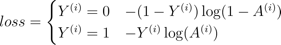
The function that has been adopted for logistic regression is the Cross-Entropy Cost Function. In the function below, Y is the ground-truth label, and A is our probabilistic label.

Notice that the function changes based on whether y is 1 or 0.
- When y = 1, the function computes the log of the label. If the prediction is correct, the loss will be 0 (i.e., log(1) = 0). If it’s incorrect, the loss will get larger and larger as the prediction approaches 0.
- When y = 0, the function subtracts 1 from y and then computes the log of the label. This subtraction keeps the loss low for correct predictions and high for incorrect predictions.
Let’s now populate our function to compute the cross-entropy cost for an input data array.
2.4 Gradient Descent
Now that we can compute the cost of the model, we must use the cost to ‘tune’ the model’s parameters via gradient descent. If you need a refresher on gradient descent, check out my Breaking it Down: Gradient Descent post.
Let’s create a fake scenario: imagine that we are training a model to predict if an adult is tired. Our fake model only gets two input features: height and hours spent awake. To accurately predict if an adult is tired, the model should probably develop a very small weight for the height feature, and a much larger weight for the hours spent awake feature.
Gradient descent will step these parameters down their gradient such that their new values will produce smaller costs. Remember, gradient descent minimizes the output of a function. We can visualize our imaginary example below.

To compute the gradient of the cost function w.r.t. the Weights and the bias, we’ll have to implement the chain rule. To find the gradients of our parameters, we’ll differentiate the cost function and the sigmoid function to find their product. We’ll then differentiate the linear function w.r.t the Weights and bias function separately.
Let’s explore a visual proof of the partial differentiations for logistic regression:
Let’s implement these simplified equations to compute the average gradients for each parameter across the training examples.
Finally, we’ve constructed all of the necessary components for our model, so now we need to integrate them. We’ll create a function that is compatible with both batch and mini-batch gradient descent.
- In batch gradient descent, every training sample is used to update the model’s parameters.
- In mini-batch gradient descent, a random portion of the training samples is selected to update the parameters. Mini-batch selection isn’t that important here, but it’s extremely useful when training data are too large to fit into the GPU/RAM.
As a reminder, fitting the model is a three-step iterative process:
- Apply linear transformation to input data with the Weights and Bias
- Apply non-linear sigmoid transformation to acquire a probabilistic label.
- Compute the gradients of the cost function w.r.t W and b and step these parameters down their gradients.
Let’s build the function!
To make sure we’re not just creating a model in isolation, let’s train the model with an example human dataset. In the context of clinical health, the model we’ll train could improve physician awareness of patient health risks.
Let’s learn by example with the UCI Heart Disease Dataset.
The dataset contains 13 features about the cardiac and physical health of adult patients. Each sample is also labeled to indicate whether the subject does or does not have heart disease.
To start, we’ll load the dataset, inspect it for missing data, and examine our feature columns. Importantly, the labels are reversed in this dataset (i.e., 1=no disease, 0=disease) so we’ll have to fix that.
Number of subjects: 303
Percentage of subjects diagnosed with heart disease:  45.54%
Number of NaN values in the dataset: 0
Let’s also visualize the features. I’ve created custom figures, but see my gist here to create your own with Seaborn.

From our inspection, we can conclude that there are no obvious missing features. We can also see that there are some stark group separations in several of the features, including age (age), exercise-induced angina (exang), chest pain (cp), and ECG shapes during exercise (oldpeak & slope). These data will be good to train a logit model!
To conclude this section, we’ll finish preparing the dataset. First, we’ll do a 75/25 split on the data to create test and train sets. Then we’ll standardize* the continuous features listed below.
to_standardize = ["age", "trestbps", "chol", "thalach", "oldpeak"]
*You don’t have to standardize data for logit models unless you’re running some form of regularization. I do it here just as a best practice.
4. Training and Testing Our Classifier
Now that we’ve built the model and prepared our dataset, let’s train our model to predict health labels.
We’ll instantiate the model, train it with our x_train and y_train data, and we’ll test it with the x_test and y_test data.
Final model cost: 0.36
Model test prediction accuracy: 86.84%
And there we have it: a test set accuracy of 86.8%. This is much better than a 50% random chance, and for such a simple model, the accuracy is quite high.
To inspect things a bit more closely, let’s visualize the model’s features during its training. On the top row, we can see the model’s cost and accuracy during its training. Then on the bottom row, we can see how the Weights and bias parameters change during training (my favorite part!).
5. Implementing Logistic Regression with TensorFlow
In the real world, it’s not best practice to build your own model when you need to use one. Instead, we can rely on powerful and well-designed open-source packages like TensorFlow, PyTorch, or scikit-learn for our ML/DL needs.
Below, let’s see how simple it is to build a logit model with TensorFlow and compare its training/test results to our own. We’ll prepare the data, create a single-layer and single-unit model with a sigmoid activation, and we’ll compile it with a binary cross-entropy loss function. Lastly, we’ll fit and evaluate the model.
Epoch 5000/5000
1/1 [==============================] - 0s 3ms/step - loss: 0.3464 - accuracy: 0.8634Test Set Accuracy:
1/1 [==============================] - 0s 191ms/step - loss: 0.3788 - accuracy: 0.8553
[0.3788422644138336, 0.8552631735801697]
From this, we can see that the model’s final training cost was 0.34 (compared to our 0.36), and the test set accuracy was 85.5%, very similar to our result above. There are a few minor differences under the hood, but the model performances are very similar.
Importantly, the TensorFlow model was built, trained, and tested in less than 25 lines of code, as opposed to our 200+ lines of code in thelogit_model.py script.
In this post, we’ve explored all of the individual aspects of the logistic regression. We started the post by building a model from scratch with NumPy. We first implemented the linear and sigmoid transformations, implemented the binary-cross entropy loss function, and created a fitting function to train our model with input data.
To understand the purpose of logistic regression, we then training our NumPy model on the UCI Heart Disease Dataset to predict heart disease in patients. We found saw the simple model had an 86% prediction accuracy — pretty impressive.
Finally, after taking the time to learn and understand these fundamentals, we then saw how easy it was to build a logit model with TensorFlow.
In sum, logistic regression is both a useful algorithm for predictive analysis. Understanding this model is a powerful first step in the road of studying deep learning.
Exploring the fundamentals of logistic regression with NumPy, TensorFlow, and the UCI Heart Disease Dataset

Outline:
1. What is Logistic Regression?
2. Breaking Down Logistic Regression
1. Linear Transformation
2. Sigmoid Activation
3. Cross-Entropy Loss Function
4. Gradient Descent
5. Fitting the Model
3. Learning by Example with the UCI Heart Disease Dataset
4. Training and Testing Our Classifier
5. Implementing Logistic Regression with TensorFlow
6. Summary
7. Notes and Resources
Logistic regression is a supervised machine learning algorithm that creates classification labels for sets of input data (1, 2). Logistic regression (logit) models are used in a variety of contexts, including healthcare, research, and business analytics.
Understanding the logic behind logistic regression can provide strong foundational insight into the basics of deep learning.
In this article, we’ll break down logistic regression to gain a fundamental understanding of the concept. To do this, we will:
- Explore the fundamental components of logistic regression and build a model from scratch with NumPy
- Train our model on the UCI Heart Disease Dataset to predict whether adults have heart disease based on their input health data
- Build a ‘formal’ logit model with TensorFlow
You can follow the code in this post with my walkthrough Jupyter Notebook and Python script files in my GitHub learning-repo.
Logistic regression models create probabilistic labels for sets of input data. These labels are often binary (yes/no).
Let’s work through an example to highlight the major aspects of logistic regression, and then we’ll start our deep dive:
Imagine that we have a logit model that’s been trained to predict if someone has diabetes. The input data to the model are a person’s age, height, weight, and blood glucose. To make its prediction, the model will transform these input data using the logistic function. The output of this function will be a probabilistic label between 0 and 1. The closer this label is to 1, the greater the model’s confidence that the person has diabetes, and vice versa.
Importantly: to create classification labels, our diabetes logit model first had to learn how to weigh the importance of each piece of input data. It’s probable that someone’s blood glucose should be weighted higher than their height for predicting diabetes. This learning occurred using a set of labeled test data and gradient descent. The learned information is stored in the model in the form of Weights and bias parameter values used in the logistic function.
This example provided a satellite-view outline of what logistic regression models do and how they work. We’re now ready for our deep dive.
To start our deep dive, let’s break down the core component of logistic regression: the logistic function.
Rather than just learning from reading alone, we’ll build our own logit model from scratch with NumPy. This will be the model’s outline:
In sections 2.1 and 2.2, we’ll implement the linear and sigmoid transformation functions.
In 2.3 we’ll define the cross-entropy cost function to tell the model when its predictions are ‘good’ and ‘bad’. In section 2.4 we’ll help the model learn its parameters via gradient descent.
Finally, in section 2.5, we’ll tie all of these functions together.
2.1 Linear Transformation
As we saw above, the logistic function first applies a linear transformation to the input data using its learned parameters: the Weights and bias.
The Weights (W) parameters indicate how important each piece of input data is to the classification. The closer an individual weight is to 0, the less important the corresponding piece of data is to the classification. The dot product of the Weights vector and input data X flattens the data into a single scalar that we can place onto a number line.
For example, if we’re trying to predict whether someone is tired based on their height and the hours they’ve spent awake, the weight for that person’s height would be very close to zero.
The bias (b) parameter is used to shift this scalar along the decision boundary of this line (0).
Let’s visualize how the linear component of the logistic function uses its learned weights and bias to transform input data from the UCI Heart Disease Dataset.
We’re now ready to start populating our model’s functions. To start, we need to initialize our model with its Weights and bias parameters. The Weights parameter will be an (n, 1) shaped array, where n is equal to the number of features in the input data. The bias parameter is a scalar. Both parameters will be initialized to 0.
Next, we can populate the function to compute the linear portion of the logistic function.
2.2 Sigmoid Activation
Logistic models create probabilistic labels (ŷ) by applying the sigmoid function to the output data from the logistic function’s linear transformation. The sigmoid function is useful to create probabilities from input data because it squishes input data to produce values between 0 and 1.
The sigmoid function is the inverse of the logit function, hence the name, logistic regression.
To create binary labels from the output of the sigmoid function, we define our decision boundary to be 0.5. This means that if ŷ ≥ 0.5, we say the label is positive, and when ŷ < 0.5, we say the label is negative.
Let’s visualize how the sigmoid function transforms the input data from the linear component of the logistic function.
Now, let’s implement this function into our model.
2.3 Cross-Entropy Cost Function
To teach our model how to optimize its Weights and bias parameters, we will feed in training data. However, for the model to learn optimal parameters, it must know how to tell if its parameters did a ‘good’ or ‘bad’ job at producing probabilistic labels.
This ‘goodness’ factor, or the difference between the probability label and the ground-truth label, is called the loss for individual samples. We operationally say that losses should be high if the parameters did a bad job at predicting the label and low if they did a good job.
The losses across the training data are then averaged to create a cost.
The function that has been adopted for logistic regression is the Cross-Entropy Cost Function. In the function below, Y is the ground-truth label, and A is our probabilistic label.
Notice that the function changes based on whether y is 1 or 0.
- When y = 1, the function computes the log of the label. If the prediction is correct, the loss will be 0 (i.e., log(1) = 0). If it’s incorrect, the loss will get larger and larger as the prediction approaches 0.
- When y = 0, the function subtracts 1 from y and then computes the log of the label. This subtraction keeps the loss low for correct predictions and high for incorrect predictions.
Let’s now populate our function to compute the cross-entropy cost for an input data array.
2.4 Gradient Descent
Now that we can compute the cost of the model, we must use the cost to ‘tune’ the model’s parameters via gradient descent. If you need a refresher on gradient descent, check out my Breaking it Down: Gradient Descent post.
Let’s create a fake scenario: imagine that we are training a model to predict if an adult is tired. Our fake model only gets two input features: height and hours spent awake. To accurately predict if an adult is tired, the model should probably develop a very small weight for the height feature, and a much larger weight for the hours spent awake feature.
Gradient descent will step these parameters down their gradient such that their new values will produce smaller costs. Remember, gradient descent minimizes the output of a function. We can visualize our imaginary example below.
To compute the gradient of the cost function w.r.t. the Weights and the bias, we’ll have to implement the chain rule. To find the gradients of our parameters, we’ll differentiate the cost function and the sigmoid function to find their product. We’ll then differentiate the linear function w.r.t the Weights and bias function separately.
Let’s explore a visual proof of the partial differentiations for logistic regression:
Let’s implement these simplified equations to compute the average gradients for each parameter across the training examples.
Finally, we’ve constructed all of the necessary components for our model, so now we need to integrate them. We’ll create a function that is compatible with both batch and mini-batch gradient descent.
- In batch gradient descent, every training sample is used to update the model’s parameters.
- In mini-batch gradient descent, a random portion of the training samples is selected to update the parameters. Mini-batch selection isn’t that important here, but it’s extremely useful when training data are too large to fit into the GPU/RAM.
As a reminder, fitting the model is a three-step iterative process:
- Apply linear transformation to input data with the Weights and Bias
- Apply non-linear sigmoid transformation to acquire a probabilistic label.
- Compute the gradients of the cost function w.r.t W and b and step these parameters down their gradients.
Let’s build the function!
To make sure we’re not just creating a model in isolation, let’s train the model with an example human dataset. In the context of clinical health, the model we’ll train could improve physician awareness of patient health risks.
Let’s learn by example with the UCI Heart Disease Dataset.
The dataset contains 13 features about the cardiac and physical health of adult patients. Each sample is also labeled to indicate whether the subject does or does not have heart disease.
To start, we’ll load the dataset, inspect it for missing data, and examine our feature columns. Importantly, the labels are reversed in this dataset (i.e., 1=no disease, 0=disease) so we’ll have to fix that.
Number of subjects: 303
Percentage of subjects diagnosed with heart disease:  45.54%
Number of NaN values in the dataset: 0
Let’s also visualize the features. I’ve created custom figures, but see my gist here to create your own with Seaborn.
From our inspection, we can conclude that there are no obvious missing features. We can also see that there are some stark group separations in several of the features, including age (age), exercise-induced angina (exang), chest pain (cp), and ECG shapes during exercise (oldpeak & slope). These data will be good to train a logit model!
To conclude this section, we’ll finish preparing the dataset. First, we’ll do a 75/25 split on the data to create test and train sets. Then we’ll standardize* the continuous features listed below.
to_standardize = ["age", "trestbps", "chol", "thalach", "oldpeak"]
*You don’t have to standardize data for logit models unless you’re running some form of regularization. I do it here just as a best practice.
4. Training and Testing Our Classifier
Now that we’ve built the model and prepared our dataset, let’s train our model to predict health labels.
We’ll instantiate the model, train it with our x_train and y_train data, and we’ll test it with the x_test and y_test data.
Final model cost: 0.36
Model test prediction accuracy: 86.84%
And there we have it: a test set accuracy of 86.8%. This is much better than a 50% random chance, and for such a simple model, the accuracy is quite high.
To inspect things a bit more closely, let’s visualize the model’s features during its training. On the top row, we can see the model’s cost and accuracy during its training. Then on the bottom row, we can see how the Weights and bias parameters change during training (my favorite part!).
5. Implementing Logistic Regression with TensorFlow
In the real world, it’s not best practice to build your own model when you need to use one. Instead, we can rely on powerful and well-designed open-source packages like TensorFlow, PyTorch, or scikit-learn for our ML/DL needs.
Below, let’s see how simple it is to build a logit model with TensorFlow and compare its training/test results to our own. We’ll prepare the data, create a single-layer and single-unit model with a sigmoid activation, and we’ll compile it with a binary cross-entropy loss function. Lastly, we’ll fit and evaluate the model.
Epoch 5000/5000
1/1 [==============================] - 0s 3ms/step - loss: 0.3464 - accuracy: 0.8634Test Set Accuracy:
1/1 [==============================] - 0s 191ms/step - loss: 0.3788 - accuracy: 0.8553
[0.3788422644138336, 0.8552631735801697]
From this, we can see that the model’s final training cost was 0.34 (compared to our 0.36), and the test set accuracy was 85.5%, very similar to our result above. There are a few minor differences under the hood, but the model performances are very similar.
Importantly, the TensorFlow model was built, trained, and tested in less than 25 lines of code, as opposed to our 200+ lines of code in thelogit_model.py script.
In this post, we’ve explored all of the individual aspects of the logistic regression. We started the post by building a model from scratch with NumPy. We first implemented the linear and sigmoid transformations, implemented the binary-cross entropy loss function, and created a fitting function to train our model with input data.
To understand the purpose of logistic regression, we then training our NumPy model on the UCI Heart Disease Dataset to predict heart disease in patients. We found saw the simple model had an 86% prediction accuracy — pretty impressive.
Finally, after taking the time to learn and understand these fundamentals, we then saw how easy it was to build a logit model with TensorFlow.
In sum, logistic regression is both a useful algorithm for predictive analysis. Understanding this model is a powerful first step in the road of studying deep learning.
Denial of responsibility! Techno Blender is an automatic aggregator of the all world’s media. In each content, the hyperlink to the primary source is specified. All trademarks belong to their rightful owners, all materials to their authors. If you are the owner of the content and do not want us to publish your materials, please contact us by email – [email protected]. The content will be deleted within 24 hours.