
Build Complex Time Series Regression Pipelines with sktime | by Rhys Kilian | Jul, 2022
How to forecast with scikit-learn and XGBoost models with sktime
Stop using scikit-learn for forecasting. Just because you can use your existing regression pipeline doesn’t mean you should. Alternatively, aren’t you bored of forecasting using the same old techniques, such as exponential smoothing and ARIMA? Wouldn’t it be more fun to use a more advanced algorithm such as a gradient boosted tree?
Using sktime, you can do this (and more). Sktime is a library that lets you safely use any scikit-learn compatible regression model for time series forecasting. This tutorial will discuss how we can convert a time series forecasting problem to a regression problem using sktime. I will also show you how to build a complex time series forecaster with the popular library, XGBoost.
What is time series forecasting?
Time series forecasting is a technique to predict one or more future values. Like regression modelling, a data practitioner can fit a model based on historical data and use this model to predict future observations.
Some of the most popular models used in forecasting are univariate. Univariate models forecast using only the previous observations. Exponential smoothing models use a weighted average of past observations to predict future values, with more recent data points given more weight. ARIMA models base their predictions on the autocorrelations in the data. Autocorrelation measures the relationship between time-shifted (i.e. lagged) values of a time series.
If time series forecasting sounds similar to regression modelling, you’re correct. We can use regression models for our time-series predictions.
Why would we want to use regression for time series forecasting?
One of the reasons you should use regression models is for improved model performance. Regression techniques are flexible, and you can go beyond univariate modelling of past observations. Including time-step features, such as the day of the week or holidays, can enrich your data and potentially uncover hidden trends in your data.
Secondly, you likely already use popular machine learning frameworks such as scikit-learn and XGBoost. Converting your time series forecasting task into a regression problem can save you time if you’re already familiar with these libraries.
However, modern forecasting libraries, such as Facebook’s Prophet, also provide the flexibility for multivariate analysis and a simple API. Nonetheless, using regression techniques for forecasting should be another tool in your data science toolkit.
What do we need to watch out for in time series regression?
Time series regression isn’t without issues. Autocorrelated observations violate the assumptions of linear regression models. However, more complex regression models, such as gradient tree boosting, are generally robust to multicollinearity.
Additionally, we can introduce data leakage if we blindly fit and tune our regression model. Data leakage is the use of information in the model training and validation phase that would not otherwise be available for forecasting. For example, randomly shuffling your data using K-fold cross-validation allows your model to peek ahead into the future. Instead, you should use temporal cross-validation.
Rather than implementing time-series regression models from scratch, you can use the sktime framework.
Why should we use sktime?
Sktime is an open-source framework for various machine learning tasks for modelling time series, including time-series regression, classification, clustering and annotation. The framework combines features from several libraries with a user experience similar to scikit-learn.
We will be using sktime for our forecasting task because it provides functionality such as:
- Reduction: building a time series forecaster using estimators compatible with the scikit-learn API
- Tuning: determining the value of hyperparameters using grid search strategies with temporal cross-validation
- Evaluation: sktime includes several performance metrics (e.g. MAPE, MASE) and provides an easy implementation for custom scorers and backtesting
- Pipelining: an extension of the scikit-learn Pipeline, which is a series of concatenated transformers to build a single forecaster
- AutoML: automated tuning strategies to determine the best forecaster across a range of models and hyperparameters
Sktime also provides several other classes of forecasting models, including exponential smoothing, ARIMA, BATS and Prophet. We will not discuss these forecasting models in this tutorial, but I encourage you to implement these forecasters during your model selection phase.
Dataset
The dataset we will be using in this tutorial is an hourly count of pedestrians in the city of Melbourne, Australia [1]. We will restrict our analysis from 1st January 2010 to 31st December 2019. I’ve aggregated the data weekly.
If we visualise our data, we can see a general upwards trend from about mid-2013. We can also see more pedestrians in the city in December, likely due to Christmas shopping, and in July for end-of-financial-year sales. Our data appears non-stationary, confirmed when we run an Augmented Dickey-Fuller test.

A simple forecaster with linear regression
The first example we’ll run is a simple forecaster using linear regression. We first take the final 26 weeks of data as our test set using sktime’s temporal_train_test_split. The function does not shuffle the data. Therefore it is suitable for forecasting.
from sktime.forecasting.model_selection import temporal_train_test_splity_train, y_test = temporal_train_test_split(y, test_size=26)
We also specify our forecasting horizon, the 26 weeks of test data that we will predict. We achieve this using the ForecastingHorizon object.
from sktime.forecasting.base import ForecastingHorizonfh = ForecastingHorizon(y_test.index, is_relative=False)
With the preliminaries complete, we can move on to instantiating our scikit-learn LinearRegression object that will be the estimator for our forecaster. Alternatively, you can use other scikit-learn estimators or scikit-learn API compatible estimators, such as XGBoost. I will demonstrate this in the following example.
from sklearn.linear_model import LinearRegressionregressor = LinearRegression()
Sktime’s make_reduction function transforms the time series into tabular data compatible with our scikit-learn estimator. The parameter, ‘window_length’, controls the number of lags in our sliding window transformation.
Consider the simple time series, denoted ‘y’, below. If we apply our make_reduction function, with a window length equal to 3, we produce a tabular dataset with three input variables, denoted ‘lag_1’, ‘lag_2’ and ‘lag_3’. The function transforms our one-dimensional time series dataset into a compatible format with our regression estimator.

Furthermore, the make_reduction function has an input ‘strategy’, which controls how the forecaster generates its predictions. The parameter is relevant when we are making more than one-step ahead forecasts. In our example, we are making predictions for the next 26 weeks of pedestrian counts (multi-step) rather than just the following week (one-step).
We have the choice of three options for our multi-step forecasting strategy:
- Direct: we create a separate model for each period we are forecasting. In our example, we fit 26 models, each making a single prediction.
- Recursive: we fit a single one-step ahead model. However, we use the previous time step’s output for the following input. For example, we use next week’s prediction as an input for the prediction two weeks away, and so on.
- Multiple outputs: one model is used to predict the entire time series horizon in a single forecast. The use of this option is dependent on having a model capable of predicting sequences.
In our example, we will use the recursive strategy.
from sktime.forecasting.compose import make_reductionforecaster = make_reduction(regressor, window_length=52, strategy="recursive")
We can now fit our linear regression forecaster and predict the 26 weeks of pedestrian counts on our test data.
forecaster.fit(y_train)
y_pred = forecaster.predict(fh)
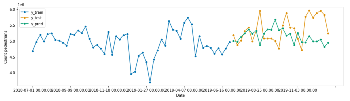
We then plot our predictions relative to the train and test data to determine the model’s suitability. Sktime makes this easy using the plot_series utility function.
from sktime.utils.plotting import plot_seriesplot_series(y_train['2018-07-01':], y_test, y_pred, labels=["y_train", "y_test", "y_pred"], x_label='Date', y_label='Count pedestrians');

Our linear regression forecaster appears to give us a reasonable fit. However, it is a conservative prediction and misses the peaks and troughs of the test data.
We evaluate our model using the mean_absolute_percentage_error (MAPE), which yields a result of 4.8%.
from sktime.performance_metrics.forecasting import mean_absolute_percentage_errorprint('MAPE: %.4f' % mean_absolute_percentage_error(y_test, y_pred, symmetric=False))
If we put all this together, our code looks like this:
Let’s see if we can beat this using a more complex algorithm such as XGBoost.
Time series forecasting with XGBoost and exogenous inputs
XGBoost is an implementation of a gradient boosting machine, popular for tabular machine learning tasks because of its speed and performance. We can use XGBoost for time series forecasting because it has a scikit-learn wrapper compatible with sktime’s make_reduction function.
from xgboost import XGBRegressorregressor = XGBRegressor(objective='reg:squarederror', random_state=42)
forecaster = make_reduction(regressor, window_length=52, strategy="recursive")
We will also include exogenous data, another time helpful series for the prediction that is not forecasted. Let’s include several dummy variables that indicate the year’s month, split into our train and test sets.
# Create an exogenous dataframe indicating the month
X = pd.DataFrame({'month': y.index.month}, index=y.index)
X = pd.get_dummies(X.astype(str), drop_first=True)# Split into train and test
X_train, X_test = temporal_train_test_split(X, test_size=26)
We include our exogenous data when we call the fit and predict methods. You can find more information in the RecursiveTabularRegressionForecaster documentation.
forecaster.fit(y=y_train, X=X_train)
y_pred = forecaster.predict(fh=fh, X=X_test)
Visually, our predictions appear to be worse than our linear regression forecaster. Our expectation is confirmed when we look at the MAPE, which has increased to 7.1%. The XGBoost forecaster is likely under-fitted because we’ve used the default hyperparameter values.
The following example will demonstrate how we can tune the hyperparameters for our XGBoost forecaster.

You can find the code for this example below.
Tuning the hyperparameters of our forecaster
Our XGBRegressor has several hyperparameters that we can tune, as described in this article. We want to adjust the hyperparameters of our forecaster to see if we can improve the performance.
Before tuning our hyperparameters, we must add a validation set to our data. We have several strategies implemented by sktime, including a SingleWindowSplitter, SlidingWindowSplitter, and ExpandingWindowSplitter. For simplicity, we will create a single validation set, the same size as our test set. However, this article explains the differences between the various strategies.
from sktime.forecasting.model_selection import SingleWindowSplittervalidation_size = 26
cv = SingleWindowSplitter(window_length=len(y)-validation_size, fh=validation_size)
Sktime has implemented two strategies for hyperparameter tuning: randomised search and grid search. We will use a randomised search with 100 iterations.
from sktime.forecasting.model_selection import ForecastingRandomizedSearchCVparam_grid = {
'estimator__max_depth': [3, 5, 6, 10, 15, 20],
'estimator__learning_rate': [0.01, 0.1, 0.2, 0.3],
'estimator__subsample': np.arange(0.5, 1.0, 0.1),
'estimator__colsample_bytree': np.arange(0.4, 1.0, 0.1),
'estimator__colsample_bylevel': np.arange(0.4, 1.0, 0.1),
'estimator__n_estimators': [100, 500, 1000]
}regressor = XGBRegressor(objective='reg:squarederror', random_state=42)
forecaster = make_reduction(regressor, window_length=52, strategy="recursive")gscv = ForecastingRandomizedSearchCV(forecaster, cv=cv, param_distributions=param_grid, n_iter=100, random_state=42)
Again, we fit and predict.
gscv.fit(y=y_train, X=X_train)
y_pred = gscv.predict(fh=fh, X=X_test)
But this time, we can inspect our random search object to see how the forecaster performs using different combinations of hyperparameters.
gscv.cv_results_
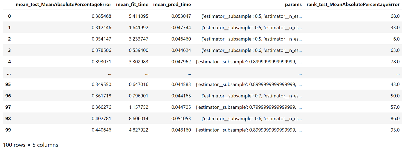
Interestingly, our forecaster performs worse on our test data, as shown by our visualisation and the MAPE increasing to 7.8%.
You can find the complete code for the example below.
Adding components to our forecasting pipeline
We previously trained our model on non-stationary data resulting in a poor forecast. Using statsmodels, we can decompose our pedestrian time series to observe the trend and seasonality.
from statsmodels.tsa.seasonal import seasonal_decomposeresult = seasonal_decompose(y_train, model='multiplicative')
result.plot()
plt.show()
We assume our time series is multiplicative rather than additive because it appears the oscillation amplitude of our time series increases over time. Looking at the decomposition below, we see that our trend (second subplot) has increased since mid-2013 and that there is a seasonal pattern, with increased pedestrian traffic around Christmas and mid-year and decreased traffic in the first week of January.

Therefore, our forecaster’s performance may be improved by removing the seasonality and trend of the time series, producing a time series closer to being stationary. Sktime includes two classes, Deseasonalizer and Detrender, that we can incorporate into our forecasting pipeline.
from sktime.forecasting.compose import TransformedTargetForecaster
from sktime.transformations.series.detrend import Deseasonalizer, Detrender
from sktime.forecasting.trend import PolynomialTrendForecasterregressor = XGBRegressor(objective='reg:squarederror', random_state=42)forecaster = TransformedTargetForecaster(
[
("deseasonalize", Deseasonalizer(model="multiplicative", sp=52)),
("detrend", Detrender(forecaster=PolynomialTrendForecaster(degree=1))),
("forecast", make_reduction(regressor, window_length=52, strategy="recursive"),
),
]
)
We can tune the parameters for our Deaseasonalizer and Detrender using a randomised grid search. For example, we can see if an additive or multiplicative model is best or what degree of the polynomial we want to use to model the trend.
param_grid = {
'deseasonalize__model': ['multiplicative', 'additive'],
'detrend__forecaster__degree': [1, 2, 3],
'forecast__estimator__max_depth': [3, 5, 6, 10, 15, 20],
'forecast__estimator__learning_rate': [0.01, 0.1, 0.2, 0.3],
'forecast__estimator__subsample': np.arange(0.5, 1.0, 0.1),
'forecast__estimator__colsample_bytree': np.arange(0.4, 1.0, 0.1),
'forecast__estimator__colsample_bylevel': np.arange(0.4, 1.0, 0.1),
'forecast__estimator__n_estimators': [100, 500, 1000]
}gscv = ForecastingRandomizedSearchCV(forecaster, cv=cv, param_distributions=param_grid, n_iter=100, random_state=42)
gscv.fit(y=y_train, X=X_train)
y_pred = gscv.predict(fh=fh, X=X_test)
After tuning our forecaster pipeline, we can visualise our predictions. We observe our predictions are much closer to our trend data, indicating that removing the seasonality and trend from our time series has improved the performance of our model. The MAPE has decreased to 4.7%, the best performance of all our models tested.

The complete code for this example is below.
How to forecast with scikit-learn and XGBoost models with sktime
Stop using scikit-learn for forecasting. Just because you can use your existing regression pipeline doesn’t mean you should. Alternatively, aren’t you bored of forecasting using the same old techniques, such as exponential smoothing and ARIMA? Wouldn’t it be more fun to use a more advanced algorithm such as a gradient boosted tree?
Using sktime, you can do this (and more). Sktime is a library that lets you safely use any scikit-learn compatible regression model for time series forecasting. This tutorial will discuss how we can convert a time series forecasting problem to a regression problem using sktime. I will also show you how to build a complex time series forecaster with the popular library, XGBoost.
What is time series forecasting?
Time series forecasting is a technique to predict one or more future values. Like regression modelling, a data practitioner can fit a model based on historical data and use this model to predict future observations.
Some of the most popular models used in forecasting are univariate. Univariate models forecast using only the previous observations. Exponential smoothing models use a weighted average of past observations to predict future values, with more recent data points given more weight. ARIMA models base their predictions on the autocorrelations in the data. Autocorrelation measures the relationship between time-shifted (i.e. lagged) values of a time series.
If time series forecasting sounds similar to regression modelling, you’re correct. We can use regression models for our time-series predictions.
Why would we want to use regression for time series forecasting?
One of the reasons you should use regression models is for improved model performance. Regression techniques are flexible, and you can go beyond univariate modelling of past observations. Including time-step features, such as the day of the week or holidays, can enrich your data and potentially uncover hidden trends in your data.
Secondly, you likely already use popular machine learning frameworks such as scikit-learn and XGBoost. Converting your time series forecasting task into a regression problem can save you time if you’re already familiar with these libraries.
However, modern forecasting libraries, such as Facebook’s Prophet, also provide the flexibility for multivariate analysis and a simple API. Nonetheless, using regression techniques for forecasting should be another tool in your data science toolkit.
What do we need to watch out for in time series regression?
Time series regression isn’t without issues. Autocorrelated observations violate the assumptions of linear regression models. However, more complex regression models, such as gradient tree boosting, are generally robust to multicollinearity.
Additionally, we can introduce data leakage if we blindly fit and tune our regression model. Data leakage is the use of information in the model training and validation phase that would not otherwise be available for forecasting. For example, randomly shuffling your data using K-fold cross-validation allows your model to peek ahead into the future. Instead, you should use temporal cross-validation.
Rather than implementing time-series regression models from scratch, you can use the sktime framework.
Why should we use sktime?
Sktime is an open-source framework for various machine learning tasks for modelling time series, including time-series regression, classification, clustering and annotation. The framework combines features from several libraries with a user experience similar to scikit-learn.
We will be using sktime for our forecasting task because it provides functionality such as:
- Reduction: building a time series forecaster using estimators compatible with the scikit-learn API
- Tuning: determining the value of hyperparameters using grid search strategies with temporal cross-validation
- Evaluation: sktime includes several performance metrics (e.g. MAPE, MASE) and provides an easy implementation for custom scorers and backtesting
- Pipelining: an extension of the scikit-learn Pipeline, which is a series of concatenated transformers to build a single forecaster
- AutoML: automated tuning strategies to determine the best forecaster across a range of models and hyperparameters
Sktime also provides several other classes of forecasting models, including exponential smoothing, ARIMA, BATS and Prophet. We will not discuss these forecasting models in this tutorial, but I encourage you to implement these forecasters during your model selection phase.
Dataset
The dataset we will be using in this tutorial is an hourly count of pedestrians in the city of Melbourne, Australia [1]. We will restrict our analysis from 1st January 2010 to 31st December 2019. I’ve aggregated the data weekly.
If we visualise our data, we can see a general upwards trend from about mid-2013. We can also see more pedestrians in the city in December, likely due to Christmas shopping, and in July for end-of-financial-year sales. Our data appears non-stationary, confirmed when we run an Augmented Dickey-Fuller test.
A simple forecaster with linear regression
The first example we’ll run is a simple forecaster using linear regression. We first take the final 26 weeks of data as our test set using sktime’s temporal_train_test_split. The function does not shuffle the data. Therefore it is suitable for forecasting.
from sktime.forecasting.model_selection import temporal_train_test_splity_train, y_test = temporal_train_test_split(y, test_size=26)
We also specify our forecasting horizon, the 26 weeks of test data that we will predict. We achieve this using the ForecastingHorizon object.
from sktime.forecasting.base import ForecastingHorizonfh = ForecastingHorizon(y_test.index, is_relative=False)
With the preliminaries complete, we can move on to instantiating our scikit-learn LinearRegression object that will be the estimator for our forecaster. Alternatively, you can use other scikit-learn estimators or scikit-learn API compatible estimators, such as XGBoost. I will demonstrate this in the following example.
from sklearn.linear_model import LinearRegressionregressor = LinearRegression()
Sktime’s make_reduction function transforms the time series into tabular data compatible with our scikit-learn estimator. The parameter, ‘window_length’, controls the number of lags in our sliding window transformation.
Consider the simple time series, denoted ‘y’, below. If we apply our make_reduction function, with a window length equal to 3, we produce a tabular dataset with three input variables, denoted ‘lag_1’, ‘lag_2’ and ‘lag_3’. The function transforms our one-dimensional time series dataset into a compatible format with our regression estimator.
Furthermore, the make_reduction function has an input ‘strategy’, which controls how the forecaster generates its predictions. The parameter is relevant when we are making more than one-step ahead forecasts. In our example, we are making predictions for the next 26 weeks of pedestrian counts (multi-step) rather than just the following week (one-step).
We have the choice of three options for our multi-step forecasting strategy:
- Direct: we create a separate model for each period we are forecasting. In our example, we fit 26 models, each making a single prediction.
- Recursive: we fit a single one-step ahead model. However, we use the previous time step’s output for the following input. For example, we use next week’s prediction as an input for the prediction two weeks away, and so on.
- Multiple outputs: one model is used to predict the entire time series horizon in a single forecast. The use of this option is dependent on having a model capable of predicting sequences.
In our example, we will use the recursive strategy.
from sktime.forecasting.compose import make_reductionforecaster = make_reduction(regressor, window_length=52, strategy="recursive")
We can now fit our linear regression forecaster and predict the 26 weeks of pedestrian counts on our test data.
forecaster.fit(y_train)
y_pred = forecaster.predict(fh)
We then plot our predictions relative to the train and test data to determine the model’s suitability. Sktime makes this easy using the plot_series utility function.
from sktime.utils.plotting import plot_seriesplot_series(y_train['2018-07-01':], y_test, y_pred, labels=["y_train", "y_test", "y_pred"], x_label='Date', y_label='Count pedestrians');
Our linear regression forecaster appears to give us a reasonable fit. However, it is a conservative prediction and misses the peaks and troughs of the test data.
We evaluate our model using the mean_absolute_percentage_error (MAPE), which yields a result of 4.8%.
from sktime.performance_metrics.forecasting import mean_absolute_percentage_errorprint('MAPE: %.4f' % mean_absolute_percentage_error(y_test, y_pred, symmetric=False))
If we put all this together, our code looks like this:
Let’s see if we can beat this using a more complex algorithm such as XGBoost.
Time series forecasting with XGBoost and exogenous inputs
XGBoost is an implementation of a gradient boosting machine, popular for tabular machine learning tasks because of its speed and performance. We can use XGBoost for time series forecasting because it has a scikit-learn wrapper compatible with sktime’s make_reduction function.
from xgboost import XGBRegressorregressor = XGBRegressor(objective='reg:squarederror', random_state=42)
forecaster = make_reduction(regressor, window_length=52, strategy="recursive")
We will also include exogenous data, another time helpful series for the prediction that is not forecasted. Let’s include several dummy variables that indicate the year’s month, split into our train and test sets.
# Create an exogenous dataframe indicating the month
X = pd.DataFrame({'month': y.index.month}, index=y.index)
X = pd.get_dummies(X.astype(str), drop_first=True)# Split into train and test
X_train, X_test = temporal_train_test_split(X, test_size=26)
We include our exogenous data when we call the fit and predict methods. You can find more information in the RecursiveTabularRegressionForecaster documentation.
forecaster.fit(y=y_train, X=X_train)
y_pred = forecaster.predict(fh=fh, X=X_test)
Visually, our predictions appear to be worse than our linear regression forecaster. Our expectation is confirmed when we look at the MAPE, which has increased to 7.1%. The XGBoost forecaster is likely under-fitted because we’ve used the default hyperparameter values.
The following example will demonstrate how we can tune the hyperparameters for our XGBoost forecaster.
You can find the code for this example below.
Tuning the hyperparameters of our forecaster
Our XGBRegressor has several hyperparameters that we can tune, as described in this article. We want to adjust the hyperparameters of our forecaster to see if we can improve the performance.
Before tuning our hyperparameters, we must add a validation set to our data. We have several strategies implemented by sktime, including a SingleWindowSplitter, SlidingWindowSplitter, and ExpandingWindowSplitter. For simplicity, we will create a single validation set, the same size as our test set. However, this article explains the differences between the various strategies.
from sktime.forecasting.model_selection import SingleWindowSplittervalidation_size = 26
cv = SingleWindowSplitter(window_length=len(y)-validation_size, fh=validation_size)
Sktime has implemented two strategies for hyperparameter tuning: randomised search and grid search. We will use a randomised search with 100 iterations.
from sktime.forecasting.model_selection import ForecastingRandomizedSearchCVparam_grid = {
'estimator__max_depth': [3, 5, 6, 10, 15, 20],
'estimator__learning_rate': [0.01, 0.1, 0.2, 0.3],
'estimator__subsample': np.arange(0.5, 1.0, 0.1),
'estimator__colsample_bytree': np.arange(0.4, 1.0, 0.1),
'estimator__colsample_bylevel': np.arange(0.4, 1.0, 0.1),
'estimator__n_estimators': [100, 500, 1000]
}regressor = XGBRegressor(objective='reg:squarederror', random_state=42)
forecaster = make_reduction(regressor, window_length=52, strategy="recursive")gscv = ForecastingRandomizedSearchCV(forecaster, cv=cv, param_distributions=param_grid, n_iter=100, random_state=42)
Again, we fit and predict.
gscv.fit(y=y_train, X=X_train)
y_pred = gscv.predict(fh=fh, X=X_test)
But this time, we can inspect our random search object to see how the forecaster performs using different combinations of hyperparameters.
gscv.cv_results_
Interestingly, our forecaster performs worse on our test data, as shown by our visualisation and the MAPE increasing to 7.8%.
You can find the complete code for the example below.
Adding components to our forecasting pipeline
We previously trained our model on non-stationary data resulting in a poor forecast. Using statsmodels, we can decompose our pedestrian time series to observe the trend and seasonality.
from statsmodels.tsa.seasonal import seasonal_decomposeresult = seasonal_decompose(y_train, model='multiplicative')
result.plot()
plt.show()
We assume our time series is multiplicative rather than additive because it appears the oscillation amplitude of our time series increases over time. Looking at the decomposition below, we see that our trend (second subplot) has increased since mid-2013 and that there is a seasonal pattern, with increased pedestrian traffic around Christmas and mid-year and decreased traffic in the first week of January.
Therefore, our forecaster’s performance may be improved by removing the seasonality and trend of the time series, producing a time series closer to being stationary. Sktime includes two classes, Deseasonalizer and Detrender, that we can incorporate into our forecasting pipeline.
from sktime.forecasting.compose import TransformedTargetForecaster
from sktime.transformations.series.detrend import Deseasonalizer, Detrender
from sktime.forecasting.trend import PolynomialTrendForecasterregressor = XGBRegressor(objective='reg:squarederror', random_state=42)forecaster = TransformedTargetForecaster(
[
("deseasonalize", Deseasonalizer(model="multiplicative", sp=52)),
("detrend", Detrender(forecaster=PolynomialTrendForecaster(degree=1))),
("forecast", make_reduction(regressor, window_length=52, strategy="recursive"),
),
]
)
We can tune the parameters for our Deaseasonalizer and Detrender using a randomised grid search. For example, we can see if an additive or multiplicative model is best or what degree of the polynomial we want to use to model the trend.
param_grid = {
'deseasonalize__model': ['multiplicative', 'additive'],
'detrend__forecaster__degree': [1, 2, 3],
'forecast__estimator__max_depth': [3, 5, 6, 10, 15, 20],
'forecast__estimator__learning_rate': [0.01, 0.1, 0.2, 0.3],
'forecast__estimator__subsample': np.arange(0.5, 1.0, 0.1),
'forecast__estimator__colsample_bytree': np.arange(0.4, 1.0, 0.1),
'forecast__estimator__colsample_bylevel': np.arange(0.4, 1.0, 0.1),
'forecast__estimator__n_estimators': [100, 500, 1000]
}gscv = ForecastingRandomizedSearchCV(forecaster, cv=cv, param_distributions=param_grid, n_iter=100, random_state=42)
gscv.fit(y=y_train, X=X_train)
y_pred = gscv.predict(fh=fh, X=X_test)
After tuning our forecaster pipeline, we can visualise our predictions. We observe our predictions are much closer to our trend data, indicating that removing the seasonality and trend from our time series has improved the performance of our model. The MAPE has decreased to 4.7%, the best performance of all our models tested.
The complete code for this example is below.
Denial of responsibility! Techno Blender is an automatic aggregator of the all world’s media. In each content, the hyperlink to the primary source is specified. All trademarks belong to their rightful owners, all materials to their authors. If you are the owner of the content and do not want us to publish your materials, please contact us by email – [email protected]. The content will be deleted within 24 hours.