
Building A Graph Convolutional Network for Molecular Property Prediction
Artificial Intelligence
Tutorial to make molecular graphs and develop a simple PyTorch-based GCN
Artificial intelligence has taken the world by storm. Every week, new models, tools, and applications emerge that promise to push the boundaries of human endeavor. The availability of open-source tools that enable users to train and employ complex machine learning models in a modest number of lines of code have truly democratized AI; at the same time, while many of these off-the-shelf models may provide excellent predictive capabilities, their usage as black box models may deprive inquisitive students of AI of a deeper understanding of how they work and why they were developed in the first place. This understanding is particularly important in the natural sciences, where knowing that a model is accurate is not enough — it is also essential to know its connection to other physical theories, its limitations, and its generalizability to other systems. In this article, we will explore the basics of one particular ML model — a graph convolutional network — through the lens of chemistry. This is not meant to be a mathematically rigorous exploration; instead, we will try to compare features of the network with traditional models in the natural sciences and think about why it works as well as it does.
1. The need for graphs and graph neural networks
A model in chemistry or physics is usually a continuous function, say y=f(x₁, x₂, x₃, …, xₙ), in which x₁, x₂, x₃, …, xₙ are the inputs and y is the output. An example of such a model is the equation that determines the electrostatic interaction (or force) between two point charges q₁ and q₂ separated by a distance r present in a medium with relative permittivity εᵣ, commonly termed as Coulomb’s law.
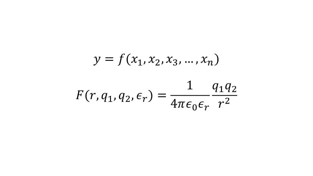
If we did not know this relationship but, hypothetically, had multiple datapoints each including the interaction between point charges (the output) and the corresponding inputs, we could fit an artificial neural network to predict the interaction for any given point charges for any given separation in a medium with a specified permittivity. In the case of this problem, admittedly ignoring some important caveats, creating a data-driven model for a physical problem is relatively straightforward.
Now consider the problem of prediction of a particular property, say solubility in water, from the structure of a molecule. First, there is no obvious set of inputs to describe a molecule. You could use various features, such as bond lengths, bond angles, number of different types of elements, number of rings, and so forth. However, there is no guarantee that any such arbitrary set is bound to work well for all molecules.
Second, unlike the example of the point charges, the inputs may not necessarily reside in a continuous space. For example, we can think of methanol, ethanol, and propanol as a set of molecules with increasing chain lengths; there is no notion, however, of anything between them — chain length is a discrete parameter and there is no way to interpolate between methanol and ethanol to get other molecules. Having a continuous space of inputs is essential to calculate derivatives of the model, which can then be used for optimization of the chosen property.
To overcome these problems, various methods for encoding molecules have been proposed. One such method is textual representation using schemes such as SMILES and SELFIES. There is a large body of literature on this representation, and I direct the interested reader to this helpful review. The second method involves representing molecules as graphs. While each method has its advantages and shortcomings, graph representations feel more intuitive for chemistry.
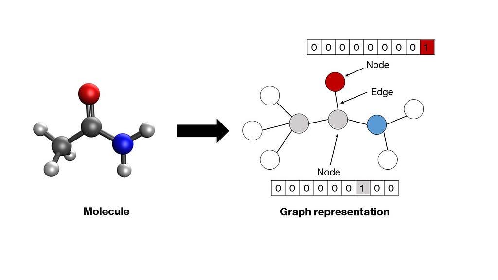
A graph is a mathematical structure consisting of nodes connected by edges that represent relationships between nodes. Molecules fit naturally into this structure — atoms become nodes, and bonds become edges. Each node in the graph is represented by a vector that encodes properties of the corresponding atom. Usually, a one-hot encoding scheme suffices (more on this in the next section). These vectors can be stacked to create a node matrix. Relationships between nodes — denoted by edges — can be delineated through a square adjacency matrix, wherein every element aᵢⱼ is either 1 or 0 depending on whether the two nodes i and j are connected by an edge or not respectively. The diagonal elements are set to 1, indicating a self-connection, which makes the matrix amenable to convolutions (as you will see in the next section). More complex graph representations can be developed, in which edge properties are also one-hot encoded in a separate matrix, but we shall leave that for another article. These node and adjacency matrices will serve as inputs to our model.
Typically, artificial neural network models accept a 1-dimensional vector of inputs. For multidimensional inputs, such as images, a class of models called convolutional neural networks was developed. In our case too we have 2-dimensional matrices as inputs, and therefore, need a modified network that can accept these as inputs. Graph neural networks were developed to operate on such node and adjacency matrices to convert them into appropriate 1-dimensional vectors that can then be passed through hidden layers of a vanilla artificial neural network to generate outputs. There are many types of graph neural networks, such as graph convolutional networks, message passing networks, graph attention networks, and so forth, which primarily differ in terms of the functions that exchange information between the nodes and edges in the graph. We shall take a closer look at graph convolutional networks due to their relative simplicity.
2. Graph convolution and pooling layers
Consider the initial state of your inputs. The node matrix represents the one-hot encoding of each atom in each row. For the sake of simplicity, let us consider a one-hot encoding of atomic numbers, wherein an atom with atomic number n will have a 1 at the nᵗʰ index and 0s everywhere else. The adjacency matrix represents the connections between the nodes. In its current state, the node matrix cannot be used as an input to an artificial neural network for the following reasons: (1) it is 2-dimensional, (2) it is not permutation-invariant, and (3) it is not unique. Permutation-invariance in this case implies that the input should remain the same no matter how you order the nodes; currently, the same molecule can be represented by multiple permutations of the same node matrix (assuming an appropriate permutation in the adjacency matrix as well). This is a problem since the network would treat different permutations as different inputs, when they should be treated as the same.
There is an easy solution to the first two issues — pooling. If the node matrix is pooled along the column dimension, then it will be reduced to a 1-dimensional vector that is permutation-invariant. Typically, this pooling is a simple mean pooling, which means that the final pooled vector contains the means of every column in the node matrix. However, this still does not solve the third problem — pooling the node matrices of two isomers, such as n-pentane and neo-pentane, will produce the same pooled vector.
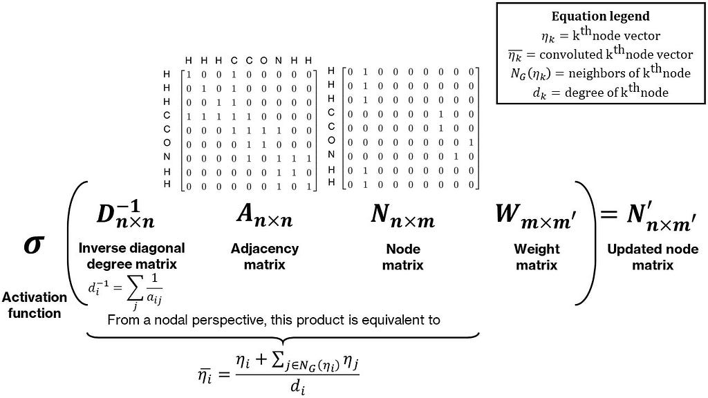
To make the final pooled vectors unique, we need to incorporate some neighbor information in the node matrix. In the case of isomers, while their chemical formula is the same, their structure is not. A simple way to incorporate neighbor information is to perform some operation, such as a sum, for each node with its neighbors. This can be represented as the multiplication of the node and adjacency matrices (try it out on paper: the adjacency matrix times the node matrix produces an updated node matrix with each node vector equal to the sum of its neighbor node vectors with itself). Often, this sum is normalized by the degree (or number of neighbors) of each node by pre-multiplying with the inverse of the diagonal degree matrix, making this a mean over neighbors. Lastly, this product is post-multiplied by a weight matrix to make this operation parameterizable. This whole operation is termed as a graph convolution. An intuitive and simple form of a graph convolution is shown in Figure 3. A more mathematically rigorous and numerically stable form was provided in Thomas Kipf and Max Welling’s work, with a modified normalization of the adjacency matrix. The combination of convolution and pooling operations can also be interpreted as a non-linear form of an empirical group contribution method.
The final structure of the graph convolutional network is as follows — first, node and adjacency matrices are calculated for a given molecule. Multiple graph convolutions are then applied to these followed by pooling to produce a single vector containing all the information regarding the molecule. This is then passed through the hidden layers of a standard artificial neural network to produce an output. The weights of the hidden layers, pooling layer, and convolution layers are simultaneously determined through backpropagation applied to a regression-based loss function like mean-squared loss.
3. Implementation in code
Having discussed all the key ideas related to graph convolutional networks, we are ready to start building one using PyTorch. While there exists a flexible, high-performance framework for GNNs called PyTorch Geometric, we shall not make use of it, since our goal is to look under the hood and develop our understanding.
The tutorial is split into four major subsections — (1) creating graphs in an automated fashion using RDKit, (2) packaging the graphs into a PyTorch Dataset, (3) building the graph convolutional network architecture, and (4) training the network. The complete code, along with instructions to install and import the required packages, is provided in a GitHub repository with a link at the end of the article.
3.1. Creating graphs using RDKit
RDKit is a cheminformatics library that allows high-throughput access to properties of small molecules. We will need it for two tasks — getting the atomic number of each atom in a molecule to one-hot encode the node matrix and getting the adjacency matrix. We assume that molecules are provided in terms of their SMILES strings (which is true for most cheminformatics data). Additionally, to ensure that the sizes of node and adjacency matrices are uniform across all molecules — which they would not be by default, since the sizes of both are dependent on the number of atoms in a molecule — we pad the matrices with 0s. Finally, we shall try a small modification to the convolution that we have proposed above — we will replace the “1”s in the adjacency matrix with the reciprocals of the corresponding bond lengths. This way, the network will have more information regarding the geometry of the molecule, and it will also weight the convolutions around each node based on the bond lengths of the neighbors.
class Graph:
    def __init__(
        self, molecule_smiles: str,
        node_vec_len: int,
        max_atoms: int = None
      ):
        # Store properties
        self.smiles = molecule_smiles
        self.node_vec_len = node_vec_len
        self.max_atoms = max_atoms

        # Call helper function to convert SMILES to RDKit mol
        self.smiles_to_mol()

        # If valid mol is created, generate a graph of the mol
        if self.mol is not None:
            self.smiles_to_graph()

    def smiles_to_mol(self):
        # Use MolFromSmiles from RDKit to get molecule object
        mol = Chem.MolFromSmiles(self.smiles)

        # If a valid mol is not returned, set mol as None and exit
        if mol is None:
            self.mol = None
            return

        # Add hydrogens to molecule
        self.mol = Chem.AddHs(mol)

    def smiles_to_graph(self):
        # Get list of atoms in molecule
        atoms = self.mol.GetAtoms()

        # If max_atoms is not provided, max_atoms is equal to maximum number
        # of atoms in this molecule.
        if self.max_atoms is None:
            n_atoms = len(list(atoms))
        else:
            n_atoms = self.max_atoms

        # Create empty node matrix
        node_mat = np.zeros((n_atoms, self.node_vec_len))

        # Iterate over atoms and add to node matrix
        for atom in atoms:
            # Get atom index and atomic number
            atom_index = atom.GetIdx()
            atom_no = atom.GetAtomicNum()

            # Assign to node matrix
            node_mat[atom_index, atom_no] = 1

        # Get adjacency matrix using RDKit
        adj_mat = rdmolops.GetAdjacencyMatrix(self.mol)
        self.std_adj_mat = np.copy(adj_mat)

        # Get distance matrix using RDKit
        dist_mat = molDG.GetMoleculeBoundsMatrix(self.mol)
        dist_mat[dist_mat == 0.] = 1

        # Get modified adjacency matrix with inverse bond lengths
        adj_mat = adj_mat * (1 / dist_mat)

        # Pad the adjacency matrix with 0s
        dim_add = n_atoms - adj_mat.shape[0]
        adj_mat = np.pad(
            adj_mat, pad_width=((0, dim_add), (0, dim_add)), mode="constant"
        )

        # Add an identity matrix to adjacency matrix
        # This will make an atom its own neighbor
        adj_mat = adj_mat + np.eye(n_atoms)

        # Save both matrices
        self.node_mat = node_mat
        self.adj_mat = adj_mat
3.2. Packaging graphs in a Dataset
PyTorch provides a handy Dataset class to store and access various kinds of data. We will use that to store the node and adjacency matrices and output for each molecule. Note that it is not mandatory to use this Dataset interface to handle data; nonetheless, using this abstraction makes subsequent steps simpler. We need to define two main methods for our class GraphData that inherits from the Dataset class: a __len__ method to get the size of the dataset and crucially a __getitem__ method to fetch the input and output for a given index.
class GraphData(Dataset):
    def __init__(self, dataset_path: str, node_vec_len: int, max_atoms: int):
        # Save attributes
        self.node_vec_len = node_vec_len
        self.max_atoms = max_atoms

        # Open dataset file
        df = pd.read_csv(dataset_path)

        # Create lists
        self.indices = df.index.to_list()
        self.smiles = df["smiles"].to_list()
        self.outputs = df["measured log solubility in mols per litre"].to_list()

    def __len__(self):
        return len(self.indices)

    def __getitem__(self, i: int):
        # Get smile
        smile = self.smiles[i]

        # Create MolGraph object using the Graph abstraction
        mol = Graph(smile, self.node_vec_len, self.max_atoms)

        # Get node and adjacency matrices
        node_mat = torch.Tensor(mol.node_mat)
        adj_mat = torch.Tensor(mol.adj_mat)

        # Get output
        output = torch.Tensor([self.outputs[i]])

        return (node_mat, adj_mat), output, smile
Since we have defined our own customized manner of returning the node and adjacency matrices, outputs, and SMILES strings, we need to define a custom function to collate the data, that is, package it into a batch, which is then passed on to the network. This ability to train neural networks by passing batches of data, rather than individual datapoints, and using mini-batch gradient descent provides a delicate balance between accuracy and compute efficiency. The collate function that we will define below will essentially collect all the data objects, stratify them into their categories, stack them in lists, convert them into PyTorch Tensors, and recombine these tensors such that they are returned in the same manner as that of our GraphData class.
def collate_graph_dataset(dataset: Dataset):
    # Create empty lists of node and adjacency matrices, outputs, and smiles
    node_mats = []
    adj_mats = []
    outputs = []
    smiles = []

    # Iterate over list and assign each component to the correct list
    for i in range(len(dataset)):
        (node_mat,adj_mat), output, smile = dataset[i]
        node_mats.append(node_mat)
        adj_mats.append(adj_mat)
        outputs.append(output)
        smiles.append(smile)


    # Create tensors
    node_mats_tensor = torch.cat(node_mats, dim=0)
    adj_mats_tensor = torch.cat(adj_mats, dim=0)
    outputs_tensor = torch.stack(outputs, dim=0)

    # Return tensors
    return (node_mats_tensor, adj_mats_tensor), outputs_tensor, smiles
3.3. Building the graph convolutional network architecture
Having completed the data processing aspects of the code, we now turn towards building the model itself. We shall build our own convolution and pooling layers for the sake of perspicuity, but more advanced developers among you can easily swap these out with more complex, pre-defined layers from the PyTorch Geometric module. The ConvolutionLayer essentially does three things — (1) calculation of the inverse diagonal degree matrix from the adjacency matrix, (2) multiplication of the four matrices (D⁻¹ANW), and (3) application of a non-linear activation function to the layer output. As with other PyTorch classes, we will inherit from the Module base class that already has definitions for methods like forward.
class ConvolutionLayer(nn.Module):
    def __init__(self, node_in_len: int, node_out_len: int):
        # Call constructor of base class
        super().__init__()

        # Create linear layer for node matrix
        self.conv_linear = nn.Linear(node_in_len, node_out_len)

        # Create activation function
        self.conv_activation = nn.LeakyReLU()

    def forward(self, node_mat, adj_mat):
        # Calculate number of neighbors
        n_neighbors = adj_mat.sum(dim=-1, keepdims=True)
        # Create identity tensor
        self.idx_mat = torch.eye(
            adj_mat.shape[-2], adj_mat.shape[-1], device=n_neighbors.device
        )
        # Add new (batch) dimension and expand
        idx_mat = self.idx_mat.unsqueeze(0).expand(*adj_mat.shape)
        # Get inverse degree matrix
        inv_degree_mat = torch.mul(idx_mat, 1 / n_neighbors)

        # Perform matrix multiplication: D^(-1)AN
        node_fea = torch.bmm(inv_degree_mat, adj_mat)
        node_fea = torch.bmm(node_fea, node_mat)

        # Perform linear transformation to node features
        # (multiplication with W)
        node_fea = self.conv_linear(node_fea)

        # Apply activation
        node_fea = self.conv_activation(node_fea)

        return node_fea
Next, let us construct the PoolingLayer. This layer only performs one operation, that is, a mean along the second dimension (number of nodes).
class PoolingLayer(nn.Module):
    def __init__(self):
        # Call constructor of base class
        super().__init__()

    def forward(self, node_fea):
        # Pool the node matrix
        pooled_node_fea = node_fea.mean(dim=1)
        return pooled_node_fea
Finally, we shall define create the ChemGCN class containing the definitions of convolutional, pooling, and hidden layers. Typically, this class should have a constructor that defines the structure and ordering of each of these layers, and a forward method that accepts the input (in our case, the node and adjacency matrices) and produces the output. We will apply the LeakyReLU activation function to all of the layer outputs. Also, we shall use dropout to minimize overfitting.
class ChemGCN(nn.Module):
    def __init__(
        self,
        node_vec_len: int,
        node_fea_len: int,
        hidden_fea_len: int,
        n_conv: int,
        n_hidden: int,
        n_outputs: int,
        p_dropout: float = 0.0,
    ):
        # Call constructor of base class
        super().__init__()

        # Define layers
        # Initial transformation from node matrix to node features
        self.init_transform = nn.Linear(node_vec_len, node_fea_len)

        # Convolution layers
        self.conv_layers = nn.ModuleList(
            [
                ConvolutionLayer(
                    node_in_len=node_fea_len,
                    node_out_len=node_fea_len,
                )
                for i in range(n_conv)
            ]
        )

        # Pool convolution outputs
        self.pooling = PoolingLayer()
        pooled_node_fea_len = node_fea_len

        # Pooling activation
        self.pooling_activation = nn.LeakyReLU()

        # From pooled vector to hidden layers
        self.pooled_to_hidden = nn.Linear(pooled_node_fea_len, hidden_fea_len)

        # Hidden layer
        self.hidden_layer = nn.Linear(hidden_fea_len, hidden_fea_len)

        # Hidden layer activation function
        self.hidden_activation = nn.LeakyReLU()

        # Hidden layer dropout
        self.dropout = nn.Dropout(p=p_dropout)

        # If hidden layers more than 1, add more hidden layers
        self.n_hidden = n_hidden
        if self.n_hidden > 1:
            self.hidden_layers = nn.ModuleList(
                [self.hidden_layer for _ in range(n_hidden - 1)]
            )
            self.hidden_activation_layers = nn.ModuleList(
                [self.hidden_activation for _ in range(n_hidden - 1)]
            )
            self.hidden_dropout_layers = nn.ModuleList(
                [self.dropout for _ in range(n_hidden - 1)]
            )

        # Final layer going to the output
        self.hidden_to_output = nn.Linear(hidden_fea_len, n_outputs)

    def forward(self, node_mat, adj_mat):
        # Perform initial transform on node_mat
        node_fea = self.init_transform(node_mat)

        # Perform convolutions
        for conv in self.conv_layers:
            node_fea = conv(node_fea, adj_mat)

        # Perform pooling
        pooled_node_fea = self.pooling(node_fea)
        pooled_node_fea = self.pooling_activation(pooled_node_fea)

        # First hidden layer
        hidden_node_fea = self.pooled_to_hidden(pooled_node_fea)
        hidden_node_fea = self.hidden_activation(hidden_node_fea)
        hidden_node_fea = self.dropout(hidden_node_fea)

        # Subsequent hidden layers
        if self.n_hidden > 1:
            for i in range(self.n_hidden - 1):
                hidden_node_fea = self.hidden_layers[i](hidden_node_fea)
                hidden_node_fea = self.hidden_activation_layers[i](hidden_node_fea)
                hidden_node_fea = self.hidden_dropout_layers[i](hidden_node_fea)

        # Output
        out = self.hidden_to_output(hidden_node_fea)

        return out
3.4. Training the network
We have built the tools required to train our model and make predictions. In this section, we shall write helper functions to train and test our model, and a write script to run a workflow that makes graphs, builds the network, and trains the model.
First, we shall define a Standardizer class to standardize our outputs. Neural networks like to deal with relatively small numbers that do not vary wildly from each other. Standardization helps with that.
class Standardizer:
    def __init__(self, X):
        self.mean = torch.mean(X)
        self.std = torch.std(X)

    def standardize(self, X):
        Z = (X - self.mean) / (self.std)
        return Z

    def restore(self, Z):
        X = self.mean + Z * self.std
        return X

    def state(self):
        return {"mean": self.mean, "std": self.std}

    def load(self, state):
        self.mean = state["mean"]
        self.std = state["std"]
Second, we define a function to perform the following steps per epoch:
- Unpack inputs and outputs from the data loader and transfer them to the GPU (if available).
- Pass the inputs through the network and get predictions.
- Calculate the mean-squared loss between the predictions and outputs.
- Perform backpropagation and update the weights of the network.
- Repeat the above steps for other batches.
The function returns the batch-averaged loss and mean absolute error that can be used to plot a loss curve. A similar function without the backpropagation is written to test the model.
def train_model(
    epoch,
    model,
    training_dataloader,
    optimizer,
    loss_fn,
    standardizer,
    use_GPU,
    max_atoms,
    node_vec_len,
):
    # Create variables to store losses and error
    avg_loss = 0
    avg_mae = 0
    count = 0

    # Switch model to train mode
    model.train()

    # Go over each batch in the dataloader
    for i, dataset in enumerate(training_dataloader):
        # Unpack data
        node_mat = dataset[0][0]
        adj_mat = dataset[0][1]
        output = dataset[1]

        # Reshape inputs
        first_dim = int((torch.numel(node_mat)) / (max_atoms * node_vec_len))
        node_mat = node_mat.reshape(first_dim, max_atoms, node_vec_len)
        adj_mat = adj_mat.reshape(first_dim, max_atoms, max_atoms)

        # Standardize output
        output_std = standardizer.standardize(output)

        # Package inputs and outputs; check if GPU is enabled
        if use_GPU:
            nn_input = (node_mat.cuda(), adj_mat.cuda())
            nn_output = output_std.cuda()
        else:
            nn_input = (node_mat, adj_mat)
            nn_output = output_std

        # Compute output from network
        nn_prediction = model(*nn_input)

        # Calculate loss
        loss = loss_fn(nn_output, nn_prediction)
        avg_loss += loss

        # Calculate MAE
        prediction = standardizer.restore(nn_prediction.detach().cpu())
        mae = mean_absolute_error(output, prediction)
        avg_mae += mae

        # Set zero gradients for all tensors
        optimizer.zero_grad()

        # Do backward prop
        loss.backward()

        # Update optimizer parameters
        optimizer.step()

        # Increase count
        count += 1

    # Calculate avg loss and MAE
    avg_loss = avg_loss / count
    avg_mae = avg_mae / count

    # Print stats
    print(
        "Epoch: [{0}]\tTraining Loss: [{1:.2f}]\tTraining MAE: [{2:.2f}]"\
           .format(
                    epoch, avg_loss, avg_mae
           )
    )

    # Return loss and MAE
    return avg_loss, avg_mae
Finally, let us write the overall workflow. This script will call everything we have defined above.
#### Fix seeds
np.random.seed(0)
torch.manual_seed(0)
use_GPU = torch.cuda.is_available()

#### Inputs
max_atoms = 200
node_vec_len = 60
train_size = 0.7
batch_size = 32
hidden_nodes = 60
n_conv_layers = 4
n_hidden_layers = 2
learning_rate = 0.01
n_epochs = 50

#### Start by creating dataset
main_path = Path(__file__).resolve().parent
data_path = main_path / "data" / "solubility_data.csv"
dataset = GraphData(dataset_path=data_path, max_atoms=max_atoms,
                        node_vec_len=node_vec_len)

#### Split data into training and test sets
# Get train and test sizes
dataset_indices = np.arange(0, len(dataset), 1)
train_size = int(np.round(train_size * len(dataset)))
test_size = len(dataset) - train_size

# Randomly sample train and test indices
train_indices = np.random.choice(dataset_indices, size=train_size,
                                                            replace=False)
test_indices = np.array(list(set(dataset_indices) - set(train_indices)))

# Create dataoaders
train_sampler = SubsetRandomSampler(train_indices)
test_sampler = SubsetRandomSampler(test_indices)
train_loader = DataLoader(dataset, batch_size=batch_size,
                          sampler=train_sampler,
                          collate_fn=collate_graph_dataset)
test_loader = DataLoader(dataset, batch_size=batch_size,
                         sampler=test_sampler,
                         collate_fn=collate_graph_dataset)

#### Initialize model, standardizer, optimizer, and loss function
# Model
model = ChemGCN(node_vec_len=node_vec_len, node_fea_len=hidden_nodes,
                hidden_fea_len=hidden_nodes, n_conv=n_conv_layers,
                n_hidden=n_hidden_layers, n_outputs=1, p_dropout=0.1)
# Transfer to GPU if needed
if use_GPU:
    model.cuda()

# Standardizer
outputs = [dataset[i][1] for i in range(len(dataset))]
standardizer = Standardizer(torch.Tensor(outputs))

# Optimizer
optimizer = torch.optim.Adam(model.parameters(), lr=learning_rate)

# Loss function
loss_fn = torch.nn.MSELoss()

#### Train the model
loss = []
mae = []
epoch = []
for i in range(n_epochs):
    epoch_loss, epoch_mae = train_model(
        i,
        model,
        train_loader,
        optimizer,
        loss_fn,
        standardizer,
        use_GPU,
        max_atoms,
        node_vec_len,
    )
    loss.append(epoch_loss)
    mae.append(epoch_mae)
    epoch.append(i)

#### Test the model
# Call test model function
test_loss, test_mae = test_model(model, test_loader, loss_fn, standardizer,
                                 use_GPU, max_atoms, node_vec_len)

#### Print final results
print(f"Training Loss: {loss[-1]:.2f}")
print(f"Training MAE: {mae[-1]:.2f}")
print(f"Test Loss: {test_loss:.2f}")
print(f"Test MAE: {test_mae:.2f}")
That’s it! Running this script should output the training and test losses and errors.
4. Results
A network with the given architecture and hyperparameters was trained on the solubility dataset from the open-source DeepChem repository containing water solubilities of ~1000 small molecules. The figure below shows the training loss curve and parity plot for the test set for one particular train-test stratification. The mean absolute errors on the training and test sets are 0.59 and 0.58 respectively (in log mol/l), lower than the 0.69 log mol/l for a linear model (based on predictions present in the dataset). It is no surprise that a neural network performs better than a linear regression model; nonetheless, this cursory comparison reassures us that the predictions made by our model are reasonable. Further, we accomplished this by only incorporating basic structural descriptors in the graphs — atomic numbers and bond lengths — and letting the convolutions and pooling functions build more complex relationships between these that led to the most accurate predictions of the molecular property.
5. Final remarks
This is by no means a definitive model for the chosen problem. There are many ways to improve the model including:
- optimizing the hyperparameters
- using an early-stopping strategy to find a model with the lowest validation loss
- using more complex convolution and pooling functions
- collecting more data
Nevertheless, the goal of this tutorial was to expound on the fundamentals of graph convolutional networks for chemistry through a simple example. Having acquainted yourself with the basics, the sky is the limit in your GCN model-building journey.
Repository and helpful references
- The complete code (including scripts to create figures) is provided in a GitHub repository. Instructions to install requisite modules are also provided there. The dataset used to train the model is from the open-source DeepChem repository that is under the MIT license (commercial use permitted). The raw dataset filename in the repository is delaney_processed.csv.
- Review on string representations of molecules.
- Research article on graph convolutional networks. The convolution function presented in this article is a simpler and more intuitive form of the function given in this article.
- Research article on message passing neural networks. These are more generalized and expressive graph neural networks. It can be shown that a graph convolutional network is a message passing neural network with a specific type of message function.
- Online book on deep learning for molecules. This is a great resource to learn the basics of deep learning for chemistry and apply your learnings through hands-on coding exercises.
Building A Graph Convolutional Network for Molecular Property Prediction was originally published in Towards Data Science on Medium, where people are continuing the conversation by highlighting and responding to this story.
Artificial Intelligence
Tutorial to make molecular graphs and develop a simple PyTorch-based GCN
Artificial intelligence has taken the world by storm. Every week, new models, tools, and applications emerge that promise to push the boundaries of human endeavor. The availability of open-source tools that enable users to train and employ complex machine learning models in a modest number of lines of code have truly democratized AI; at the same time, while many of these off-the-shelf models may provide excellent predictive capabilities, their usage as black box models may deprive inquisitive students of AI of a deeper understanding of how they work and why they were developed in the first place. This understanding is particularly important in the natural sciences, where knowing that a model is accurate is not enough — it is also essential to know its connection to other physical theories, its limitations, and its generalizability to other systems. In this article, we will explore the basics of one particular ML model — a graph convolutional network — through the lens of chemistry. This is not meant to be a mathematically rigorous exploration; instead, we will try to compare features of the network with traditional models in the natural sciences and think about why it works as well as it does.
1. The need for graphs and graph neural networks
A model in chemistry or physics is usually a continuous function, say y=f(x₁, x₂, x₃, …, xₙ), in which x₁, x₂, x₃, …, xₙ are the inputs and y is the output. An example of such a model is the equation that determines the electrostatic interaction (or force) between two point charges q₁ and q₂ separated by a distance r present in a medium with relative permittivity εᵣ, commonly termed as Coulomb’s law.
If we did not know this relationship but, hypothetically, had multiple datapoints each including the interaction between point charges (the output) and the corresponding inputs, we could fit an artificial neural network to predict the interaction for any given point charges for any given separation in a medium with a specified permittivity. In the case of this problem, admittedly ignoring some important caveats, creating a data-driven model for a physical problem is relatively straightforward.
Now consider the problem of prediction of a particular property, say solubility in water, from the structure of a molecule. First, there is no obvious set of inputs to describe a molecule. You could use various features, such as bond lengths, bond angles, number of different types of elements, number of rings, and so forth. However, there is no guarantee that any such arbitrary set is bound to work well for all molecules.
Second, unlike the example of the point charges, the inputs may not necessarily reside in a continuous space. For example, we can think of methanol, ethanol, and propanol as a set of molecules with increasing chain lengths; there is no notion, however, of anything between them — chain length is a discrete parameter and there is no way to interpolate between methanol and ethanol to get other molecules. Having a continuous space of inputs is essential to calculate derivatives of the model, which can then be used for optimization of the chosen property.
To overcome these problems, various methods for encoding molecules have been proposed. One such method is textual representation using schemes such as SMILES and SELFIES. There is a large body of literature on this representation, and I direct the interested reader to this helpful review. The second method involves representing molecules as graphs. While each method has its advantages and shortcomings, graph representations feel more intuitive for chemistry.
A graph is a mathematical structure consisting of nodes connected by edges that represent relationships between nodes. Molecules fit naturally into this structure — atoms become nodes, and bonds become edges. Each node in the graph is represented by a vector that encodes properties of the corresponding atom. Usually, a one-hot encoding scheme suffices (more on this in the next section). These vectors can be stacked to create a node matrix. Relationships between nodes — denoted by edges — can be delineated through a square adjacency matrix, wherein every element aᵢⱼ is either 1 or 0 depending on whether the two nodes i and j are connected by an edge or not respectively. The diagonal elements are set to 1, indicating a self-connection, which makes the matrix amenable to convolutions (as you will see in the next section). More complex graph representations can be developed, in which edge properties are also one-hot encoded in a separate matrix, but we shall leave that for another article. These node and adjacency matrices will serve as inputs to our model.
Typically, artificial neural network models accept a 1-dimensional vector of inputs. For multidimensional inputs, such as images, a class of models called convolutional neural networks was developed. In our case too we have 2-dimensional matrices as inputs, and therefore, need a modified network that can accept these as inputs. Graph neural networks were developed to operate on such node and adjacency matrices to convert them into appropriate 1-dimensional vectors that can then be passed through hidden layers of a vanilla artificial neural network to generate outputs. There are many types of graph neural networks, such as graph convolutional networks, message passing networks, graph attention networks, and so forth, which primarily differ in terms of the functions that exchange information between the nodes and edges in the graph. We shall take a closer look at graph convolutional networks due to their relative simplicity.
2. Graph convolution and pooling layers
Consider the initial state of your inputs. The node matrix represents the one-hot encoding of each atom in each row. For the sake of simplicity, let us consider a one-hot encoding of atomic numbers, wherein an atom with atomic number n will have a 1 at the nᵗʰ index and 0s everywhere else. The adjacency matrix represents the connections between the nodes. In its current state, the node matrix cannot be used as an input to an artificial neural network for the following reasons: (1) it is 2-dimensional, (2) it is not permutation-invariant, and (3) it is not unique. Permutation-invariance in this case implies that the input should remain the same no matter how you order the nodes; currently, the same molecule can be represented by multiple permutations of the same node matrix (assuming an appropriate permutation in the adjacency matrix as well). This is a problem since the network would treat different permutations as different inputs, when they should be treated as the same.
There is an easy solution to the first two issues — pooling. If the node matrix is pooled along the column dimension, then it will be reduced to a 1-dimensional vector that is permutation-invariant. Typically, this pooling is a simple mean pooling, which means that the final pooled vector contains the means of every column in the node matrix. However, this still does not solve the third problem — pooling the node matrices of two isomers, such as n-pentane and neo-pentane, will produce the same pooled vector.
To make the final pooled vectors unique, we need to incorporate some neighbor information in the node matrix. In the case of isomers, while their chemical formula is the same, their structure is not. A simple way to incorporate neighbor information is to perform some operation, such as a sum, for each node with its neighbors. This can be represented as the multiplication of the node and adjacency matrices (try it out on paper: the adjacency matrix times the node matrix produces an updated node matrix with each node vector equal to the sum of its neighbor node vectors with itself). Often, this sum is normalized by the degree (or number of neighbors) of each node by pre-multiplying with the inverse of the diagonal degree matrix, making this a mean over neighbors. Lastly, this product is post-multiplied by a weight matrix to make this operation parameterizable. This whole operation is termed as a graph convolution. An intuitive and simple form of a graph convolution is shown in Figure 3. A more mathematically rigorous and numerically stable form was provided in Thomas Kipf and Max Welling’s work, with a modified normalization of the adjacency matrix. The combination of convolution and pooling operations can also be interpreted as a non-linear form of an empirical group contribution method.
The final structure of the graph convolutional network is as follows — first, node and adjacency matrices are calculated for a given molecule. Multiple graph convolutions are then applied to these followed by pooling to produce a single vector containing all the information regarding the molecule. This is then passed through the hidden layers of a standard artificial neural network to produce an output. The weights of the hidden layers, pooling layer, and convolution layers are simultaneously determined through backpropagation applied to a regression-based loss function like mean-squared loss.
3. Implementation in code
Having discussed all the key ideas related to graph convolutional networks, we are ready to start building one using PyTorch. While there exists a flexible, high-performance framework for GNNs called PyTorch Geometric, we shall not make use of it, since our goal is to look under the hood and develop our understanding.
The tutorial is split into four major subsections — (1) creating graphs in an automated fashion using RDKit, (2) packaging the graphs into a PyTorch Dataset, (3) building the graph convolutional network architecture, and (4) training the network. The complete code, along with instructions to install and import the required packages, is provided in a GitHub repository with a link at the end of the article.
3.1. Creating graphs using RDKit
RDKit is a cheminformatics library that allows high-throughput access to properties of small molecules. We will need it for two tasks — getting the atomic number of each atom in a molecule to one-hot encode the node matrix and getting the adjacency matrix. We assume that molecules are provided in terms of their SMILES strings (which is true for most cheminformatics data). Additionally, to ensure that the sizes of node and adjacency matrices are uniform across all molecules — which they would not be by default, since the sizes of both are dependent on the number of atoms in a molecule — we pad the matrices with 0s. Finally, we shall try a small modification to the convolution that we have proposed above — we will replace the “1”s in the adjacency matrix with the reciprocals of the corresponding bond lengths. This way, the network will have more information regarding the geometry of the molecule, and it will also weight the convolutions around each node based on the bond lengths of the neighbors.
class Graph:
    def __init__(
        self, molecule_smiles: str,
        node_vec_len: int,
        max_atoms: int = None
      ):
        # Store properties
        self.smiles = molecule_smiles
        self.node_vec_len = node_vec_len
        self.max_atoms = max_atoms

        # Call helper function to convert SMILES to RDKit mol
        self.smiles_to_mol()

        # If valid mol is created, generate a graph of the mol
        if self.mol is not None:
            self.smiles_to_graph()

    def smiles_to_mol(self):
        # Use MolFromSmiles from RDKit to get molecule object
        mol = Chem.MolFromSmiles(self.smiles)

        # If a valid mol is not returned, set mol as None and exit
        if mol is None:
            self.mol = None
            return

        # Add hydrogens to molecule
        self.mol = Chem.AddHs(mol)

    def smiles_to_graph(self):
        # Get list of atoms in molecule
        atoms = self.mol.GetAtoms()

        # If max_atoms is not provided, max_atoms is equal to maximum number
        # of atoms in this molecule.
        if self.max_atoms is None:
            n_atoms = len(list(atoms))
        else:
            n_atoms = self.max_atoms

        # Create empty node matrix
        node_mat = np.zeros((n_atoms, self.node_vec_len))

        # Iterate over atoms and add to node matrix
        for atom in atoms:
            # Get atom index and atomic number
            atom_index = atom.GetIdx()
            atom_no = atom.GetAtomicNum()

            # Assign to node matrix
            node_mat[atom_index, atom_no] = 1

        # Get adjacency matrix using RDKit
        adj_mat = rdmolops.GetAdjacencyMatrix(self.mol)
        self.std_adj_mat = np.copy(adj_mat)

        # Get distance matrix using RDKit
        dist_mat = molDG.GetMoleculeBoundsMatrix(self.mol)
        dist_mat[dist_mat == 0.] = 1

        # Get modified adjacency matrix with inverse bond lengths
        adj_mat = adj_mat * (1 / dist_mat)

        # Pad the adjacency matrix with 0s
        dim_add = n_atoms - adj_mat.shape[0]
        adj_mat = np.pad(
            adj_mat, pad_width=((0, dim_add), (0, dim_add)), mode="constant"
        )

        # Add an identity matrix to adjacency matrix
        # This will make an atom its own neighbor
        adj_mat = adj_mat + np.eye(n_atoms)

        # Save both matrices
        self.node_mat = node_mat
        self.adj_mat = adj_mat
3.2. Packaging graphs in a Dataset
PyTorch provides a handy Dataset class to store and access various kinds of data. We will use that to store the node and adjacency matrices and output for each molecule. Note that it is not mandatory to use this Dataset interface to handle data; nonetheless, using this abstraction makes subsequent steps simpler. We need to define two main methods for our class GraphData that inherits from the Dataset class: a __len__ method to get the size of the dataset and crucially a __getitem__ method to fetch the input and output for a given index.
class GraphData(Dataset):
    def __init__(self, dataset_path: str, node_vec_len: int, max_atoms: int):
        # Save attributes
        self.node_vec_len = node_vec_len
        self.max_atoms = max_atoms

        # Open dataset file
        df = pd.read_csv(dataset_path)

        # Create lists
        self.indices = df.index.to_list()
        self.smiles = df["smiles"].to_list()
        self.outputs = df["measured log solubility in mols per litre"].to_list()

    def __len__(self):
        return len(self.indices)

    def __getitem__(self, i: int):
        # Get smile
        smile = self.smiles[i]

        # Create MolGraph object using the Graph abstraction
        mol = Graph(smile, self.node_vec_len, self.max_atoms)

        # Get node and adjacency matrices
        node_mat = torch.Tensor(mol.node_mat)
        adj_mat = torch.Tensor(mol.adj_mat)

        # Get output
        output = torch.Tensor([self.outputs[i]])

        return (node_mat, adj_mat), output, smile
Since we have defined our own customized manner of returning the node and adjacency matrices, outputs, and SMILES strings, we need to define a custom function to collate the data, that is, package it into a batch, which is then passed on to the network. This ability to train neural networks by passing batches of data, rather than individual datapoints, and using mini-batch gradient descent provides a delicate balance between accuracy and compute efficiency. The collate function that we will define below will essentially collect all the data objects, stratify them into their categories, stack them in lists, convert them into PyTorch Tensors, and recombine these tensors such that they are returned in the same manner as that of our GraphData class.
def collate_graph_dataset(dataset: Dataset):
    # Create empty lists of node and adjacency matrices, outputs, and smiles
    node_mats = []
    adj_mats = []
    outputs = []
    smiles = []

    # Iterate over list and assign each component to the correct list
    for i in range(len(dataset)):
        (node_mat,adj_mat), output, smile = dataset[i]
        node_mats.append(node_mat)
        adj_mats.append(adj_mat)
        outputs.append(output)
        smiles.append(smile)


    # Create tensors
    node_mats_tensor = torch.cat(node_mats, dim=0)
    adj_mats_tensor = torch.cat(adj_mats, dim=0)
    outputs_tensor = torch.stack(outputs, dim=0)

    # Return tensors
    return (node_mats_tensor, adj_mats_tensor), outputs_tensor, smiles
3.3. Building the graph convolutional network architecture
Having completed the data processing aspects of the code, we now turn towards building the model itself. We shall build our own convolution and pooling layers for the sake of perspicuity, but more advanced developers among you can easily swap these out with more complex, pre-defined layers from the PyTorch Geometric module. The ConvolutionLayer essentially does three things — (1) calculation of the inverse diagonal degree matrix from the adjacency matrix, (2) multiplication of the four matrices (D⁻¹ANW), and (3) application of a non-linear activation function to the layer output. As with other PyTorch classes, we will inherit from the Module base class that already has definitions for methods like forward.
class ConvolutionLayer(nn.Module):
    def __init__(self, node_in_len: int, node_out_len: int):
        # Call constructor of base class
        super().__init__()

        # Create linear layer for node matrix
        self.conv_linear = nn.Linear(node_in_len, node_out_len)

        # Create activation function
        self.conv_activation = nn.LeakyReLU()

    def forward(self, node_mat, adj_mat):
        # Calculate number of neighbors
        n_neighbors = adj_mat.sum(dim=-1, keepdims=True)
        # Create identity tensor
        self.idx_mat = torch.eye(
            adj_mat.shape[-2], adj_mat.shape[-1], device=n_neighbors.device
        )
        # Add new (batch) dimension and expand
        idx_mat = self.idx_mat.unsqueeze(0).expand(*adj_mat.shape)
        # Get inverse degree matrix
        inv_degree_mat = torch.mul(idx_mat, 1 / n_neighbors)

        # Perform matrix multiplication: D^(-1)AN
        node_fea = torch.bmm(inv_degree_mat, adj_mat)
        node_fea = torch.bmm(node_fea, node_mat)

        # Perform linear transformation to node features
        # (multiplication with W)
        node_fea = self.conv_linear(node_fea)

        # Apply activation
        node_fea = self.conv_activation(node_fea)

        return node_fea
Next, let us construct the PoolingLayer. This layer only performs one operation, that is, a mean along the second dimension (number of nodes).
class PoolingLayer(nn.Module):
    def __init__(self):
        # Call constructor of base class
        super().__init__()

    def forward(self, node_fea):
        # Pool the node matrix
        pooled_node_fea = node_fea.mean(dim=1)
        return pooled_node_fea
Finally, we shall define create the ChemGCN class containing the definitions of convolutional, pooling, and hidden layers. Typically, this class should have a constructor that defines the structure and ordering of each of these layers, and a forward method that accepts the input (in our case, the node and adjacency matrices) and produces the output. We will apply the LeakyReLU activation function to all of the layer outputs. Also, we shall use dropout to minimize overfitting.
class ChemGCN(nn.Module):
    def __init__(
        self,
        node_vec_len: int,
        node_fea_len: int,
        hidden_fea_len: int,
        n_conv: int,
        n_hidden: int,
        n_outputs: int,
        p_dropout: float = 0.0,
    ):
        # Call constructor of base class
        super().__init__()

        # Define layers
        # Initial transformation from node matrix to node features
        self.init_transform = nn.Linear(node_vec_len, node_fea_len)

        # Convolution layers
        self.conv_layers = nn.ModuleList(
            [
                ConvolutionLayer(
                    node_in_len=node_fea_len,
                    node_out_len=node_fea_len,
                )
                for i in range(n_conv)
            ]
        )

        # Pool convolution outputs
        self.pooling = PoolingLayer()
        pooled_node_fea_len = node_fea_len

        # Pooling activation
        self.pooling_activation = nn.LeakyReLU()

        # From pooled vector to hidden layers
        self.pooled_to_hidden = nn.Linear(pooled_node_fea_len, hidden_fea_len)

        # Hidden layer
        self.hidden_layer = nn.Linear(hidden_fea_len, hidden_fea_len)

        # Hidden layer activation function
        self.hidden_activation = nn.LeakyReLU()

        # Hidden layer dropout
        self.dropout = nn.Dropout(p=p_dropout)

        # If hidden layers more than 1, add more hidden layers
        self.n_hidden = n_hidden
        if self.n_hidden > 1:
            self.hidden_layers = nn.ModuleList(
                [self.hidden_layer for _ in range(n_hidden - 1)]
            )
            self.hidden_activation_layers = nn.ModuleList(
                [self.hidden_activation for _ in range(n_hidden - 1)]
            )
            self.hidden_dropout_layers = nn.ModuleList(
                [self.dropout for _ in range(n_hidden - 1)]
            )

        # Final layer going to the output
        self.hidden_to_output = nn.Linear(hidden_fea_len, n_outputs)

    def forward(self, node_mat, adj_mat):
        # Perform initial transform on node_mat
        node_fea = self.init_transform(node_mat)

        # Perform convolutions
        for conv in self.conv_layers:
            node_fea = conv(node_fea, adj_mat)

        # Perform pooling
        pooled_node_fea = self.pooling(node_fea)
        pooled_node_fea = self.pooling_activation(pooled_node_fea)

        # First hidden layer
        hidden_node_fea = self.pooled_to_hidden(pooled_node_fea)
        hidden_node_fea = self.hidden_activation(hidden_node_fea)
        hidden_node_fea = self.dropout(hidden_node_fea)

        # Subsequent hidden layers
        if self.n_hidden > 1:
            for i in range(self.n_hidden - 1):
                hidden_node_fea = self.hidden_layers[i](hidden_node_fea)
                hidden_node_fea = self.hidden_activation_layers[i](hidden_node_fea)
                hidden_node_fea = self.hidden_dropout_layers[i](hidden_node_fea)

        # Output
        out = self.hidden_to_output(hidden_node_fea)

        return out
3.4. Training the network
We have built the tools required to train our model and make predictions. In this section, we shall write helper functions to train and test our model, and a write script to run a workflow that makes graphs, builds the network, and trains the model.
First, we shall define a Standardizer class to standardize our outputs. Neural networks like to deal with relatively small numbers that do not vary wildly from each other. Standardization helps with that.
class Standardizer:
    def __init__(self, X):
        self.mean = torch.mean(X)
        self.std = torch.std(X)

    def standardize(self, X):
        Z = (X - self.mean) / (self.std)
        return Z

    def restore(self, Z):
        X = self.mean + Z * self.std
        return X

    def state(self):
        return {"mean": self.mean, "std": self.std}

    def load(self, state):
        self.mean = state["mean"]
        self.std = state["std"]
Second, we define a function to perform the following steps per epoch:
- Unpack inputs and outputs from the data loader and transfer them to the GPU (if available).
- Pass the inputs through the network and get predictions.
- Calculate the mean-squared loss between the predictions and outputs.
- Perform backpropagation and update the weights of the network.
- Repeat the above steps for other batches.
The function returns the batch-averaged loss and mean absolute error that can be used to plot a loss curve. A similar function without the backpropagation is written to test the model.
def train_model(
    epoch,
    model,
    training_dataloader,
    optimizer,
    loss_fn,
    standardizer,
    use_GPU,
    max_atoms,
    node_vec_len,
):
    # Create variables to store losses and error
    avg_loss = 0
    avg_mae = 0
    count = 0

    # Switch model to train mode
    model.train()

    # Go over each batch in the dataloader
    for i, dataset in enumerate(training_dataloader):
        # Unpack data
        node_mat = dataset[0][0]
        adj_mat = dataset[0][1]
        output = dataset[1]

        # Reshape inputs
        first_dim = int((torch.numel(node_mat)) / (max_atoms * node_vec_len))
        node_mat = node_mat.reshape(first_dim, max_atoms, node_vec_len)
        adj_mat = adj_mat.reshape(first_dim, max_atoms, max_atoms)

        # Standardize output
        output_std = standardizer.standardize(output)

        # Package inputs and outputs; check if GPU is enabled
        if use_GPU:
            nn_input = (node_mat.cuda(), adj_mat.cuda())
            nn_output = output_std.cuda()
        else:
            nn_input = (node_mat, adj_mat)
            nn_output = output_std

        # Compute output from network
        nn_prediction = model(*nn_input)

        # Calculate loss
        loss = loss_fn(nn_output, nn_prediction)
        avg_loss += loss

        # Calculate MAE
        prediction = standardizer.restore(nn_prediction.detach().cpu())
        mae = mean_absolute_error(output, prediction)
        avg_mae += mae

        # Set zero gradients for all tensors
        optimizer.zero_grad()

        # Do backward prop
        loss.backward()

        # Update optimizer parameters
        optimizer.step()

        # Increase count
        count += 1

    # Calculate avg loss and MAE
    avg_loss = avg_loss / count
    avg_mae = avg_mae / count

    # Print stats
    print(
        "Epoch: [{0}]\tTraining Loss: [{1:.2f}]\tTraining MAE: [{2:.2f}]"\
           .format(
                    epoch, avg_loss, avg_mae
           )
    )

    # Return loss and MAE
    return avg_loss, avg_mae
Finally, let us write the overall workflow. This script will call everything we have defined above.
#### Fix seeds
np.random.seed(0)
torch.manual_seed(0)
use_GPU = torch.cuda.is_available()

#### Inputs
max_atoms = 200
node_vec_len = 60
train_size = 0.7
batch_size = 32
hidden_nodes = 60
n_conv_layers = 4
n_hidden_layers = 2
learning_rate = 0.01
n_epochs = 50

#### Start by creating dataset
main_path = Path(__file__).resolve().parent
data_path = main_path / "data" / "solubility_data.csv"
dataset = GraphData(dataset_path=data_path, max_atoms=max_atoms,
                        node_vec_len=node_vec_len)

#### Split data into training and test sets
# Get train and test sizes
dataset_indices = np.arange(0, len(dataset), 1)
train_size = int(np.round(train_size * len(dataset)))
test_size = len(dataset) - train_size

# Randomly sample train and test indices
train_indices = np.random.choice(dataset_indices, size=train_size,
                                                            replace=False)
test_indices = np.array(list(set(dataset_indices) - set(train_indices)))

# Create dataoaders
train_sampler = SubsetRandomSampler(train_indices)
test_sampler = SubsetRandomSampler(test_indices)
train_loader = DataLoader(dataset, batch_size=batch_size,
                          sampler=train_sampler,
                          collate_fn=collate_graph_dataset)
test_loader = DataLoader(dataset, batch_size=batch_size,
                         sampler=test_sampler,
                         collate_fn=collate_graph_dataset)

#### Initialize model, standardizer, optimizer, and loss function
# Model
model = ChemGCN(node_vec_len=node_vec_len, node_fea_len=hidden_nodes,
                hidden_fea_len=hidden_nodes, n_conv=n_conv_layers,
                n_hidden=n_hidden_layers, n_outputs=1, p_dropout=0.1)
# Transfer to GPU if needed
if use_GPU:
    model.cuda()

# Standardizer
outputs = [dataset[i][1] for i in range(len(dataset))]
standardizer = Standardizer(torch.Tensor(outputs))

# Optimizer
optimizer = torch.optim.Adam(model.parameters(), lr=learning_rate)

# Loss function
loss_fn = torch.nn.MSELoss()

#### Train the model
loss = []
mae = []
epoch = []
for i in range(n_epochs):
    epoch_loss, epoch_mae = train_model(
        i,
        model,
        train_loader,
        optimizer,
        loss_fn,
        standardizer,
        use_GPU,
        max_atoms,
        node_vec_len,
    )
    loss.append(epoch_loss)
    mae.append(epoch_mae)
    epoch.append(i)

#### Test the model
# Call test model function
test_loss, test_mae = test_model(model, test_loader, loss_fn, standardizer,
                                 use_GPU, max_atoms, node_vec_len)

#### Print final results
print(f"Training Loss: {loss[-1]:.2f}")
print(f"Training MAE: {mae[-1]:.2f}")
print(f"Test Loss: {test_loss:.2f}")
print(f"Test MAE: {test_mae:.2f}")
That’s it! Running this script should output the training and test losses and errors.
4. Results
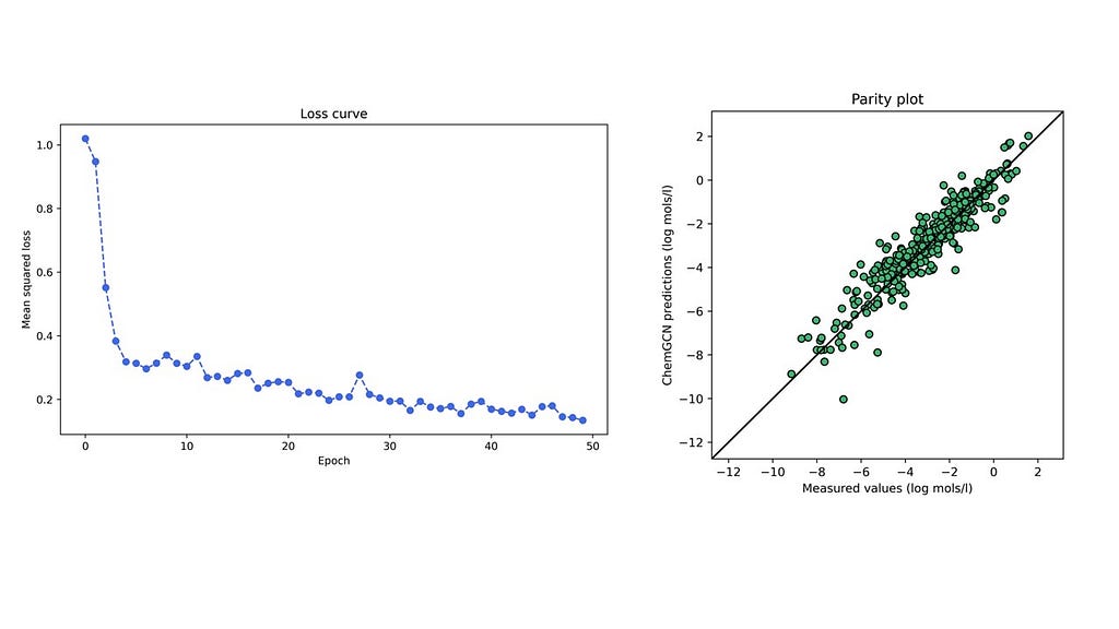
A network with the given architecture and hyperparameters was trained on the solubility dataset from the open-source DeepChem repository containing water solubilities of ~1000 small molecules. The figure below shows the training loss curve and parity plot for the test set for one particular train-test stratification. The mean absolute errors on the training and test sets are 0.59 and 0.58 respectively (in log mol/l), lower than the 0.69 log mol/l for a linear model (based on predictions present in the dataset). It is no surprise that a neural network performs better than a linear regression model; nonetheless, this cursory comparison reassures us that the predictions made by our model are reasonable. Further, we accomplished this by only incorporating basic structural descriptors in the graphs — atomic numbers and bond lengths — and letting the convolutions and pooling functions build more complex relationships between these that led to the most accurate predictions of the molecular property.
5. Final remarks
This is by no means a definitive model for the chosen problem. There are many ways to improve the model including:
- optimizing the hyperparameters
- using an early-stopping strategy to find a model with the lowest validation loss
- using more complex convolution and pooling functions
- collecting more data
Nevertheless, the goal of this tutorial was to expound on the fundamentals of graph convolutional networks for chemistry through a simple example. Having acquainted yourself with the basics, the sky is the limit in your GCN model-building journey.
Repository and helpful references
- The complete code (including scripts to create figures) is provided in a GitHub repository. Instructions to install requisite modules are also provided there. The dataset used to train the model is from the open-source DeepChem repository that is under the MIT license (commercial use permitted). The raw dataset filename in the repository is delaney_processed.csv.
- Review on string representations of molecules.
- Research article on graph convolutional networks. The convolution function presented in this article is a simpler and more intuitive form of the function given in this article.
- Research article on message passing neural networks. These are more generalized and expressive graph neural networks. It can be shown that a graph convolutional network is a message passing neural network with a specific type of message function.
- Online book on deep learning for molecules. This is a great resource to learn the basics of deep learning for chemistry and apply your learnings through hands-on coding exercises.
Building A Graph Convolutional Network for Molecular Property Prediction was originally published in Towards Data Science on Medium, where people are continuing the conversation by highlighting and responding to this story.
Denial of responsibility! Techno Blender is an automatic aggregator of the all world’s media. In each content, the hyperlink to the primary source is specified. All trademarks belong to their rightful owners, all materials to their authors. If you are the owner of the content and do not want us to publish your materials, please contact us by email – [email protected]. The content will be deleted within 24 hours.