
Building classifiers with biased classes | by Elena Jolkver | Jul, 2022
AdaSampling comes to the rescue
Leaving the world of Kaggle and entering the Real World, a data scientist is frequently (read: always) faced with the problem of dirty data. Besides missing values, different units, duplicates, and whatsoever, a rather common challenge for classification tasks is the noise in data labels. And while some noise problems can be cleaned up by the analyst, others are inherently noisy or imprecise by nature.
Consider the following task: predict whether a particular protein binds to a certain DNA sequence. Or another: predict what is causing the common cold. Both tasks have in common, that there is little knowledge about the negative class. There are zillions of DNA sequences and only those that happen to be analyzed and published as targets of the particular protein are known to be in the positive class. But the other unpublished sequences are not necessarily negative. They might just not have been analyzed. The same holds true for the common cold: many cases go undetected, as only a few people report having a cold. However, there is a technique that helps you with this challenge: Adaptive sampling, or AdaSampling, as proposed by Yang et al. (2019).
In a nutshell, the AdaSampling algorithm performs the following steps:
1. Draw a subsample from the dataset. The probability of a given positive/negative sample to be selected is equal to the probability of it being a member of the positive/negative class. (In the figure, the highlighted samples have the highest probability of being members of either class and are therefore selected for modeling.)
2. Build a classifier with any underlying classification algorithm (e.g. SVM, kNN, LDA, etc.).
3. Based on this classification model, predict the probabilities of the samples (within the complete dataset) of being in the positive/negative class.
4. Repeat 1–3 until there is no change in class probabilities.
Basically, you receive a sharpened picture of your classes and get a first clue on which of your negative samples are likely not negatives. Omitting those in your training phase can greatly increase the accuracy of your model.
Let’s try it out with the AdaSampling package in R. The example dataset is about benign and malignant breast cancers.
#install.packages("AdaSampling")
library(tidyverse)
library(AdaSampling)
library(caret)# load the example dataset
data(brca)
# some cleanup of the dataset
brca$cla <- as.factor(unlist(brca$cla))
brca$nuc <- as.numeric(as.character((brca$nuc))) #run a PCA
brca.pca <- prcomp(brca[,c(1:9)], center = TRUE,scale. = TRUE)
# append PCA components to dataset
brca_withPCA <- cbind(brca, brca.pca$x)
# plot
ggplot(brca_withPCA, aes(x=PC1, y=PC2, color=cla)) +
geom_point() +
ggtitle("PCA of Breast Cancer Dataset") +
theme_classic()
A PCA on the original dataset looks like this:
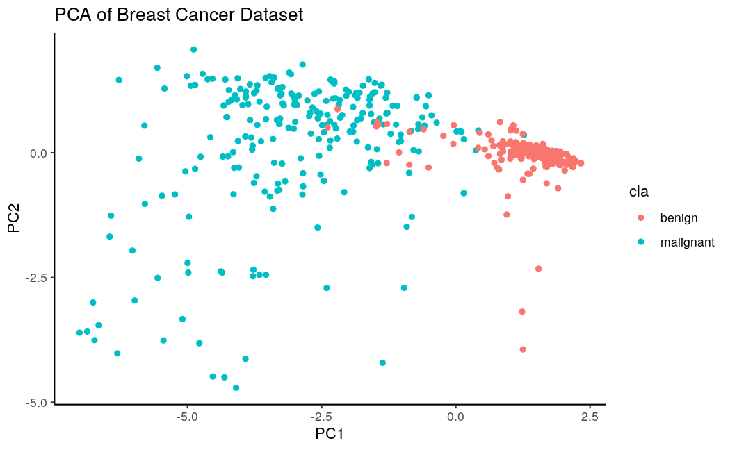
We actually see two nicely separating classes. We can build a “ground truth” classifier on it. I have picked an SVM and got an accuracy of 0.96 with a sensitivity of 0.91 (code below).
#Separate test set
set.seed(107)
inTrain <- createDataPartition(y = brca$cla,  p = 0.75)
train <- brca[ inTrain$Resample1,]
test  <- brca[-inTrain$Resample1,]ctrl <- trainControl(
method = "repeatedcv",
repeats = 3,
classProbs = TRUE,
summaryFunction = twoClassSummary
)
model_groundTruth <- train(
cla ~ .,
data = train,
method = "svmLinear", # Support Vector Machines with Linear Kernel
## Center and scale the predictors for the training
preProc = c("center", "scale"),
trControl = ctrl,
metric = "ROC"
)#predict
predicted_groundTruth <- predict(model_groundTruth, newdata = test)
confusionMatrix(data = predicted_groundTruth, test$cla, positive="malignant")
Nice. This is a pretty accurate classifier. Now let’s see AdaSampling in action. We are pretending that we move back in time and are at a time point when some of the now malignant cancers were diagnosed as benign. This is a more real-world scenario as not all cancers diagnosed as benign will stay so forever.
#get the classes
pos <- which(brca$cla == "malignant")
neg <- which(brca$cla == "benign")
#introduce 40% noise to malignant class
brca.cls <- sapply(X = brca$cla, FUN = function(x) {ifelse(x == "benign", 0, 1)})
brca.cls.noisy <- brca.cls
set.seed(1)
brca.cls.noisy[sample(pos, floor(length(neg) * 0.4))] <- 0brca$noisy_class <- as.factor(brca.cls.noisy)
brca %>% group_by(cla, noisy_class) %>% tally()

We have introduced a measurement error: 95 of cancers, which will become malignant (ground truth), are now being labeled as benign. The PCA looks quite devastating:

Building a classifier with this data results in a model with an accuracy of 0.81, sensitivity of 0.47, and specificity of 0.99. As expected, this classifier misses a lot of potentially malignant tumors.
Now it’s time for AdaSampling. The code below shows the details. The procedure is as follows: one needs to tell the algorithm which are the positive and negative samples. Then, it acts as a wrapper around a classification algorithm (I picked kNN, but the package offers many others) and reassigns the classes. Once done, I check how the sample distribution looks like with a PCA, performed on the same features as before:
# identify positive and negative examples from the noisy dataset
Ps <- rownames(brca)[which(brca$noisy_class == 1)]
Ns <- rownames(brca)[which(brca$noisy_class == 0)]# apply AdaSampling method on the noisy data. I pick kNN, but other classification methods are available
brca.preds <- adaSample(Ps, Ns, train.mat=brca[,1:9], test.mat=brca[,1:9], classifier = "knn")
brca.preds <- as.data.frame(brca.preds)
head(brca.preds)
brca.preds$Adaclass <- as.factor(ifelse(brca.preds$P > brca.preds$N, "malignant", "benign"))
brca <- cbind(brca, brca.preds["Adaclass"])#check the result with PCA first:
brca.pca_Ada <- prcomp(brca[,c(1:9)], center = TRUE,scale. = TRUE)
# append PCA components to dataset
brca_withPCA_Ada <- cbind(brca, brca.pca_Ada$x)
# plot
ggplot(brca_withPCA_Ada, aes(x=PC1, y=PC2, color=Adaclass)) +
geom_point() +
ggtitle("PCA of Breast Cancer Dataset with Noise removed by AdaSampling")+
theme_classic()

It’s almost identical to the ground truth! Just for the sake of completeness, I also build a classifier with the cleaned data, which results in a model with an accuracy of 0.96, sensitivity of 0.92, and specificity of 0.99.
The classifier is as good as the one we built on the dataset without noise. I guess this is due to the dataset and the malignant tumors were easily identifiable by the provided features. In a real-world scenario, it might look different and you can never be sure how good your model actually performs until you have gathered even more true positive and negative examples. Until then, AdaSampling is yet another tool in your toolbox for enhancing your models.
Reference: P. Yang, J. T. Ormerod, W. Liu, C. Ma, A. Y. Zomaya and J. Y. H. Yang, “AdaSampling for Positive-Unlabeled and Label Noise Learning With Bioinformatics Applications,” in IEEE Transactions on Cybernetics, vol. 49, no. 5, pp. 1932–1943, May 2019, doi: 10.1109/TCYB.2018.2816984.
AdaSampling comes to the rescue
Leaving the world of Kaggle and entering the Real World, a data scientist is frequently (read: always) faced with the problem of dirty data. Besides missing values, different units, duplicates, and whatsoever, a rather common challenge for classification tasks is the noise in data labels. And while some noise problems can be cleaned up by the analyst, others are inherently noisy or imprecise by nature.
Consider the following task: predict whether a particular protein binds to a certain DNA sequence. Or another: predict what is causing the common cold. Both tasks have in common, that there is little knowledge about the negative class. There are zillions of DNA sequences and only those that happen to be analyzed and published as targets of the particular protein are known to be in the positive class. But the other unpublished sequences are not necessarily negative. They might just not have been analyzed. The same holds true for the common cold: many cases go undetected, as only a few people report having a cold. However, there is a technique that helps you with this challenge: Adaptive sampling, or AdaSampling, as proposed by Yang et al. (2019).

In a nutshell, the AdaSampling algorithm performs the following steps:
1. Draw a subsample from the dataset. The probability of a given positive/negative sample to be selected is equal to the probability of it being a member of the positive/negative class. (In the figure, the highlighted samples have the highest probability of being members of either class and are therefore selected for modeling.)
2. Build a classifier with any underlying classification algorithm (e.g. SVM, kNN, LDA, etc.).
3. Based on this classification model, predict the probabilities of the samples (within the complete dataset) of being in the positive/negative class.
4. Repeat 1–3 until there is no change in class probabilities.
Basically, you receive a sharpened picture of your classes and get a first clue on which of your negative samples are likely not negatives. Omitting those in your training phase can greatly increase the accuracy of your model.
Let’s try it out with the AdaSampling package in R. The example dataset is about benign and malignant breast cancers.
#install.packages("AdaSampling")
library(tidyverse)
library(AdaSampling)
library(caret)# load the example dataset
data(brca)
# some cleanup of the dataset
brca$cla <- as.factor(unlist(brca$cla))
brca$nuc <- as.numeric(as.character((brca$nuc))) #run a PCA
brca.pca <- prcomp(brca[,c(1:9)], center = TRUE,scale. = TRUE)
# append PCA components to dataset
brca_withPCA <- cbind(brca, brca.pca$x)
# plot
ggplot(brca_withPCA, aes(x=PC1, y=PC2, color=cla)) +
geom_point() +
ggtitle("PCA of Breast Cancer Dataset") +
theme_classic()
A PCA on the original dataset looks like this:
We actually see two nicely separating classes. We can build a “ground truth” classifier on it. I have picked an SVM and got an accuracy of 0.96 with a sensitivity of 0.91 (code below).
#Separate test set
set.seed(107)
inTrain <- createDataPartition(y = brca$cla,  p = 0.75)
train <- brca[ inTrain$Resample1,]
test  <- brca[-inTrain$Resample1,]ctrl <- trainControl(
method = "repeatedcv",
repeats = 3,
classProbs = TRUE,
summaryFunction = twoClassSummary
)
model_groundTruth <- train(
cla ~ .,
data = train,
method = "svmLinear", # Support Vector Machines with Linear Kernel
## Center and scale the predictors for the training
preProc = c("center", "scale"),
trControl = ctrl,
metric = "ROC"
)#predict
predicted_groundTruth <- predict(model_groundTruth, newdata = test)
confusionMatrix(data = predicted_groundTruth, test$cla, positive="malignant")
Nice. This is a pretty accurate classifier. Now let’s see AdaSampling in action. We are pretending that we move back in time and are at a time point when some of the now malignant cancers were diagnosed as benign. This is a more real-world scenario as not all cancers diagnosed as benign will stay so forever.
#get the classes
pos <- which(brca$cla == "malignant")
neg <- which(brca$cla == "benign")
#introduce 40% noise to malignant class
brca.cls <- sapply(X = brca$cla, FUN = function(x) {ifelse(x == "benign", 0, 1)})
brca.cls.noisy <- brca.cls
set.seed(1)
brca.cls.noisy[sample(pos, floor(length(neg) * 0.4))] <- 0brca$noisy_class <- as.factor(brca.cls.noisy)
brca %>% group_by(cla, noisy_class) %>% tally()
We have introduced a measurement error: 95 of cancers, which will become malignant (ground truth), are now being labeled as benign. The PCA looks quite devastating:
Building a classifier with this data results in a model with an accuracy of 0.81, sensitivity of 0.47, and specificity of 0.99. As expected, this classifier misses a lot of potentially malignant tumors.
Now it’s time for AdaSampling. The code below shows the details. The procedure is as follows: one needs to tell the algorithm which are the positive and negative samples. Then, it acts as a wrapper around a classification algorithm (I picked kNN, but the package offers many others) and reassigns the classes. Once done, I check how the sample distribution looks like with a PCA, performed on the same features as before:
# identify positive and negative examples from the noisy dataset
Ps <- rownames(brca)[which(brca$noisy_class == 1)]
Ns <- rownames(brca)[which(brca$noisy_class == 0)]# apply AdaSampling method on the noisy data. I pick kNN, but other classification methods are available
brca.preds <- adaSample(Ps, Ns, train.mat=brca[,1:9], test.mat=brca[,1:9], classifier = "knn")
brca.preds <- as.data.frame(brca.preds)
head(brca.preds)
brca.preds$Adaclass <- as.factor(ifelse(brca.preds$P > brca.preds$N, "malignant", "benign"))
brca <- cbind(brca, brca.preds["Adaclass"])#check the result with PCA first:
brca.pca_Ada <- prcomp(brca[,c(1:9)], center = TRUE,scale. = TRUE)
# append PCA components to dataset
brca_withPCA_Ada <- cbind(brca, brca.pca_Ada$x)
# plot
ggplot(brca_withPCA_Ada, aes(x=PC1, y=PC2, color=Adaclass)) +
geom_point() +
ggtitle("PCA of Breast Cancer Dataset with Noise removed by AdaSampling")+
theme_classic()
It’s almost identical to the ground truth! Just for the sake of completeness, I also build a classifier with the cleaned data, which results in a model with an accuracy of 0.96, sensitivity of 0.92, and specificity of 0.99.
The classifier is as good as the one we built on the dataset without noise. I guess this is due to the dataset and the malignant tumors were easily identifiable by the provided features. In a real-world scenario, it might look different and you can never be sure how good your model actually performs until you have gathered even more true positive and negative examples. Until then, AdaSampling is yet another tool in your toolbox for enhancing your models.
Reference: P. Yang, J. T. Ormerod, W. Liu, C. Ma, A. Y. Zomaya and J. Y. H. Yang, “AdaSampling for Positive-Unlabeled and Label Noise Learning With Bioinformatics Applications,” in IEEE Transactions on Cybernetics, vol. 49, no. 5, pp. 1932–1943, May 2019, doi: 10.1109/TCYB.2018.2816984.
Denial of responsibility! Techno Blender is an automatic aggregator of the all world’s media. In each content, the hyperlink to the primary source is specified. All trademarks belong to their rightful owners, all materials to their authors. If you are the owner of the content and do not want us to publish your materials, please contact us by email – [email protected]. The content will be deleted within 24 hours.