
Cubic Splines: The Ultimate Regression Model | by Brendan Artley | Jul, 2022
Why cubic splines are the best regression model out there.
Introduction
In this article, I will go through cubic splines and show how they are more robust than high degree linear regression models. First I will walk through the mathematics behind cubic splines, then I will show the model in Python, and finally, I will explain Runge’s phenomenon.
The python library used in this article is called Regressio. This is an open source python library created by the author for univariate regression, interpolation and smoothing.
—
Firstly, a cubic spline is a piecewise interpolation model that fits a cubic polynomial to each piece in a piecewise function. At every point where 2 polynomials meet, the 1st and 2nd derivatives are equal. This makes for a smooth fitting line.

For example, in the image above we can see how a cubic polynomial could be split. In this image, there are 3 pieces, and the two central blue points are where polynomials intersect. We can see that the function is smooth around these two points and that the entire function is continuous. Let’s look at the mathematics behind fitting cubic splines.
Mathematics
Note: All the mathematical functions were created by the author of this article.
Let’s say we have three data points (2,3), (3,2), and (4,4). When calculating a cubic spline, we have to use at least 2 and at most n-1 piecewise functions. Each one of these piecewise functions are regression models to the third degree.
Since we have 3 data points, we will need 2 piecewise functions. We will denote these as f1(x) and f2(x).

In each equation above we have 4 unknown variables (a, b, c, d). We will need to set up a system of equations to calculate the unknowns in each equation, so therefore we have a total of 8 unknowns. First, we know that for the 1st and 2nd points, these points must fall on the first function.

Next, we know that the second and third points must fall on the second function.

And we also know that the 1st derivatives of two functions must be equal when they intersect.

Then, we know that the 2nd derivatives of the intersecting splines must be equal.

Finally, we want the 2nd derivatives at each endpoint to be 0. This makes a natural cubic spline.

The resulting 8 equations are as follows.

We can then plug in the three data points (2,3), (3,2), (4,4).

The equations above can then be represented in matrix form and solved using linear algebra. The equations are represented in a matrix of size 4 x (n – 1). In this example the matrix will be 8 x 8.

We can then plug these values back into our two equations and we have the piecewise functions!

It’s great that we understand the mathematics behind the algorithm, but we should not have to calculate the weights by hand each time. In the cell below I show how to solve the equation in Numpy.

Regressio Library
We can do one better than manual entry. We can use a lightweight python library called Regressio. This library has univariate models for regression, interpolation and smoothing. In the following cell we are installing the library and generating a random sample of 200 data points.

Then, we can simply import the cubic spline model and fit it to the data.

This is pretty amazing model as we can fit a highly variable relationship using a combination of low degree polynomials. Experimenting with different datasets and piecewise sizes is made easy with Regressio and I encourage you to experiment with the library. Now let’s look at why these models are better than linear regression.
Runge’s Phenomenon
Fitting spline models was exactly what Carl David Tolmé Runge was doing in 1901, and he found that polynomial interpolation methods such as cubic spline outperformed linear regression models with high degrees. This is due to large oscillations at the edges of intervals in linear regression models. This is visualized nicely in this image below.
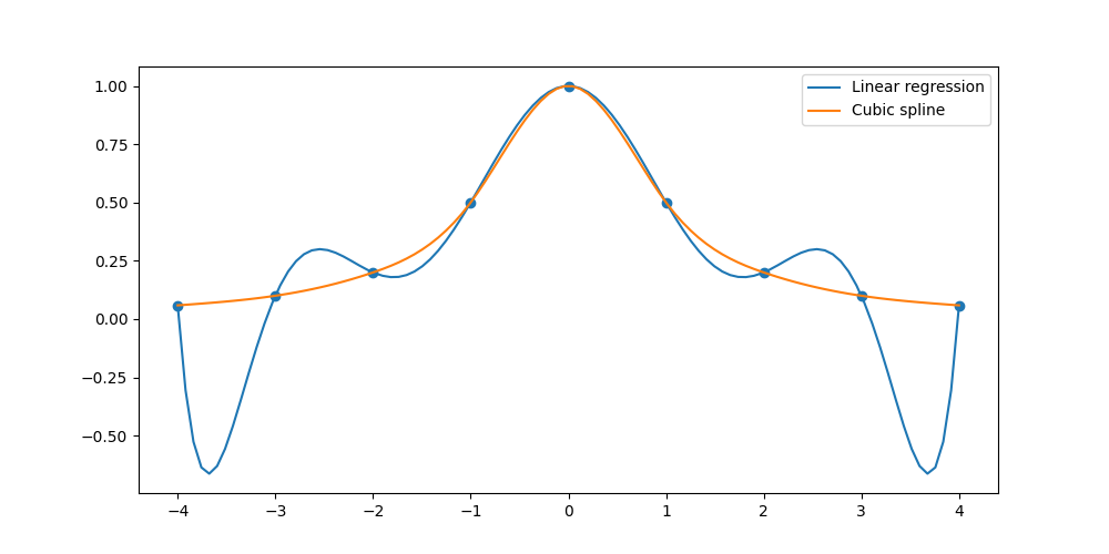
In this image, the orange line represents a cubic spline interpolation method, and the blue line represents a linear regression model. We can see the two models oscillate very differently.
For the linear regression model, if we are given a data point outside of the boundaries of the training data, then we will get an outlying prediction. This is because the magnitude of the model derivatives outside of the training range are extremely large in magnitude. This is not the case with the spline model, and why it is more robust.
Final Thoughts
Hopefully, this article showed you how cubic splines are more robust than high-degree linear regression models. Cubic splines are often skipped in introductory regression courses, but they should not be. In my opinion, they are a superior solution to linear regression models due to how they mitigate Runge’s phenomenon.
I encourage you want to work through more examples of cubic spline, and to look at other models in the Regressio library. As the author of this package, I made the code base very readable for those trying to understand how each model works. This library is still in production and is changing frequently, feel free give it a star to follow its changes, or to make contributions yourself!
If you would like the notebook code for this article, you can find that here.
References
- John, C. (2022, April 11). Runge phenomenon for interpolation at evenly spaced nodes. John D. Cook | Applied Mathematics Consulting. Retrieved July 26, 2022, from https://www.johndcook.com/blog/2017/11/18/runge-phenomena/
- Python programming and numerical methods: A guide for engineers and … University of California, Berkeley. (2021). Retrieved July 26, 2022, from https://pythonnumericalmethods.berkeley.edu/notebooks/Index.html
- Wikimedia Foundation. (2022, June 9). Runge’s phenomenon. Wikipedia. Retrieved July 26, 2022, from https://en.wikipedia.org/wiki/Runge%27s_phenomenon
Why cubic splines are the best regression model out there.

Introduction
In this article, I will go through cubic splines and show how they are more robust than high degree linear regression models. First I will walk through the mathematics behind cubic splines, then I will show the model in Python, and finally, I will explain Runge’s phenomenon.
The python library used in this article is called Regressio. This is an open source python library created by the author for univariate regression, interpolation and smoothing.
—
Firstly, a cubic spline is a piecewise interpolation model that fits a cubic polynomial to each piece in a piecewise function. At every point where 2 polynomials meet, the 1st and 2nd derivatives are equal. This makes for a smooth fitting line.
For example, in the image above we can see how a cubic polynomial could be split. In this image, there are 3 pieces, and the two central blue points are where polynomials intersect. We can see that the function is smooth around these two points and that the entire function is continuous. Let’s look at the mathematics behind fitting cubic splines.
Mathematics
Note: All the mathematical functions were created by the author of this article.
Let’s say we have three data points (2,3), (3,2), and (4,4). When calculating a cubic spline, we have to use at least 2 and at most n-1 piecewise functions. Each one of these piecewise functions are regression models to the third degree.
Since we have 3 data points, we will need 2 piecewise functions. We will denote these as f1(x) and f2(x).
In each equation above we have 4 unknown variables (a, b, c, d). We will need to set up a system of equations to calculate the unknowns in each equation, so therefore we have a total of 8 unknowns. First, we know that for the 1st and 2nd points, these points must fall on the first function.
Next, we know that the second and third points must fall on the second function.
And we also know that the 1st derivatives of two functions must be equal when they intersect.
Then, we know that the 2nd derivatives of the intersecting splines must be equal.
Finally, we want the 2nd derivatives at each endpoint to be 0. This makes a natural cubic spline.
The resulting 8 equations are as follows.
We can then plug in the three data points (2,3), (3,2), (4,4).
The equations above can then be represented in matrix form and solved using linear algebra. The equations are represented in a matrix of size 4 x (n – 1). In this example the matrix will be 8 x 8.
We can then plug these values back into our two equations and we have the piecewise functions!
It’s great that we understand the mathematics behind the algorithm, but we should not have to calculate the weights by hand each time. In the cell below I show how to solve the equation in Numpy.
Regressio Library
We can do one better than manual entry. We can use a lightweight python library called Regressio. This library has univariate models for regression, interpolation and smoothing. In the following cell we are installing the library and generating a random sample of 200 data points.
Then, we can simply import the cubic spline model and fit it to the data.
This is pretty amazing model as we can fit a highly variable relationship using a combination of low degree polynomials. Experimenting with different datasets and piecewise sizes is made easy with Regressio and I encourage you to experiment with the library. Now let’s look at why these models are better than linear regression.
Runge’s Phenomenon
Fitting spline models was exactly what Carl David Tolmé Runge was doing in 1901, and he found that polynomial interpolation methods such as cubic spline outperformed linear regression models with high degrees. This is due to large oscillations at the edges of intervals in linear regression models. This is visualized nicely in this image below.
In this image, the orange line represents a cubic spline interpolation method, and the blue line represents a linear regression model. We can see the two models oscillate very differently.
For the linear regression model, if we are given a data point outside of the boundaries of the training data, then we will get an outlying prediction. This is because the magnitude of the model derivatives outside of the training range are extremely large in magnitude. This is not the case with the spline model, and why it is more robust.
Final Thoughts
Hopefully, this article showed you how cubic splines are more robust than high-degree linear regression models. Cubic splines are often skipped in introductory regression courses, but they should not be. In my opinion, they are a superior solution to linear regression models due to how they mitigate Runge’s phenomenon.
I encourage you want to work through more examples of cubic spline, and to look at other models in the Regressio library. As the author of this package, I made the code base very readable for those trying to understand how each model works. This library is still in production and is changing frequently, feel free give it a star to follow its changes, or to make contributions yourself!
If you would like the notebook code for this article, you can find that here.
References
- John, C. (2022, April 11). Runge phenomenon for interpolation at evenly spaced nodes. John D. Cook | Applied Mathematics Consulting. Retrieved July 26, 2022, from https://www.johndcook.com/blog/2017/11/18/runge-phenomena/
- Python programming and numerical methods: A guide for engineers and … University of California, Berkeley. (2021). Retrieved July 26, 2022, from https://pythonnumericalmethods.berkeley.edu/notebooks/Index.html
- Wikimedia Foundation. (2022, June 9). Runge’s phenomenon. Wikipedia. Retrieved July 26, 2022, from https://en.wikipedia.org/wiki/Runge%27s_phenomenon
Denial of responsibility! Techno Blender is an automatic aggregator of the all world’s media. In each content, the hyperlink to the primary source is specified. All trademarks belong to their rightful owners, all materials to their authors. If you are the owner of the content and do not want us to publish your materials, please contact us by email – [email protected]. The content will be deleted within 24 hours.