
Data Analytics in Fashion: Excel Series (#2) | by Olaoluwakiitan Olabiyi | Jul, 2022
A comprehensive blueprint on getting started with data analysis in Microsoft Excel
Welcome to tutorial #2 of the Excel Series. Click HERE to read tutorial #1. Otherwise, proceed to tutorial #2 below.
The data cleaning techniques to cover in this tutorial are;
- Resize columns
- Get rid of leading and trailing spaces.
- Remove line breaks from cells
- Remove Duplicates
- Deal with blank rows and cells
- Standardize sentence case
The datasets used are fashion datasets from Kaggle and you can access them here>>> dataset 1 and dataset 2
Let’s get started!
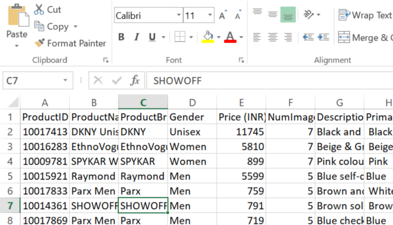
Sometimes, when you import your dataset into Excel, some of the columns appear to be squashed making it difficult to see the entire values in each cell. An example is seen in Fig. 1 below.
There are different ways to resolve this but a faster approach would involve two steps.
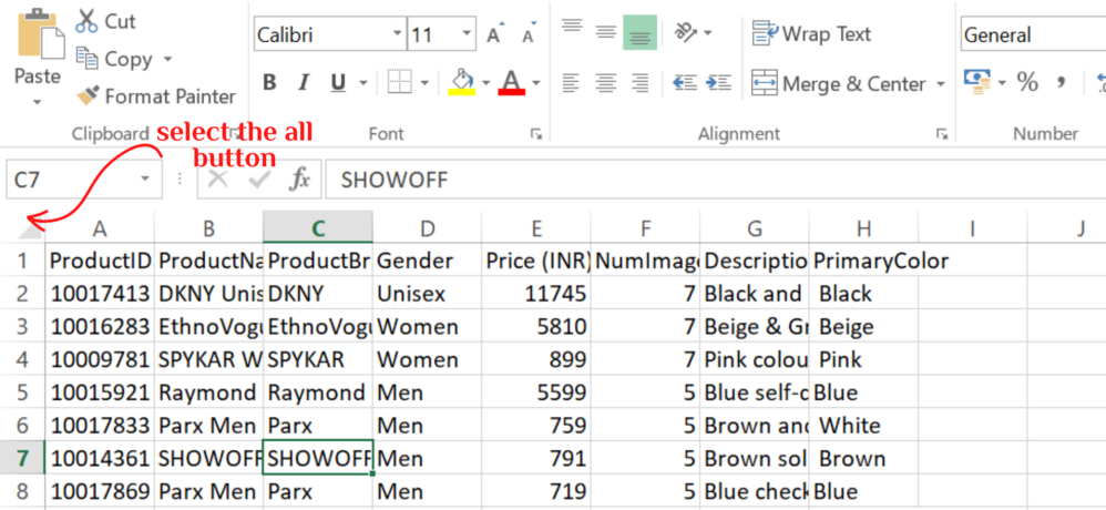
STEPS:1.Select the 'all button'(to the left of column 'A').
2.Double click on any of the boundary lines between the columns.
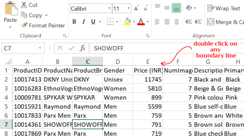
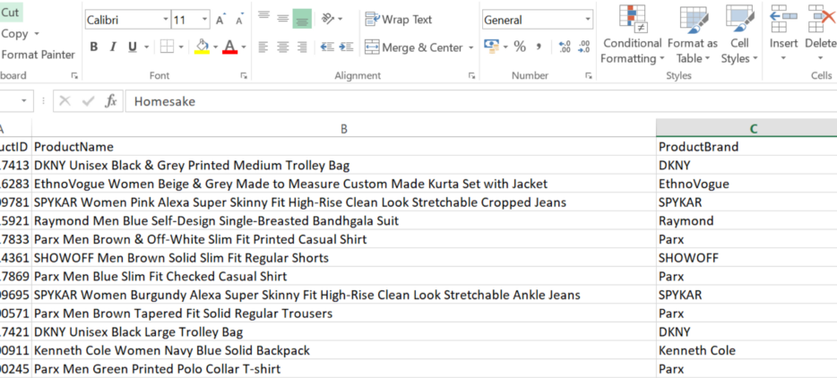
This will automatically resize all columns as shown in Fig. 4.
The same data is shown in Fig. 4 but now looks more readable.
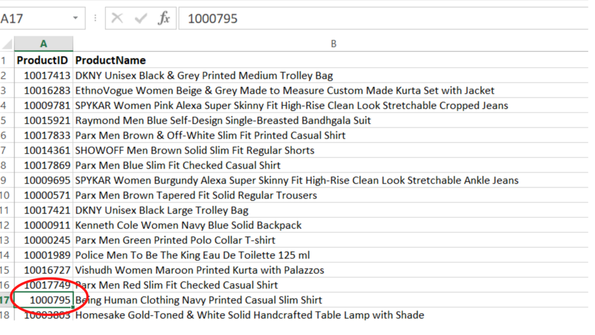
Leading and trailing spaces are unnecessary gaps that appear at the beginning, between, or end of data input and they might be difficult to spot. An example is shown in Column A, Fig. 5.
To get rid of these spaces, use the TRIM function.
Syntax:
=TRIM(text)
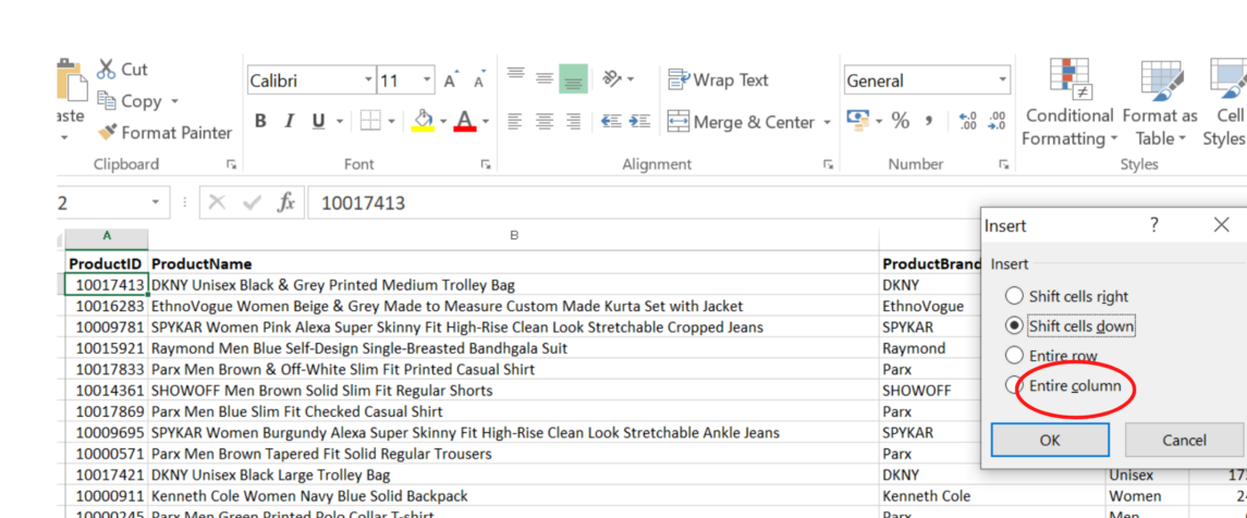
STEPS:1. Place your cursor on the column (ProductID) you wish to clean, hit Ctrl shift + at the same time.
2. Select'Entire column'as illustrated in Fig. 6a
3. Click ok.(This will create a new column to the left of ProductID).
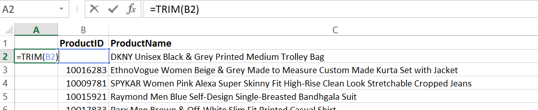
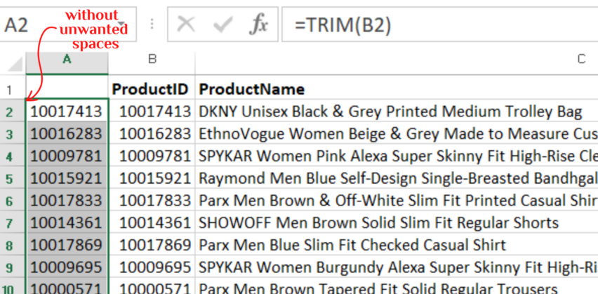
4. In the new column(column A),Type =TRIM(B2);where B2 is the cell reference for ProductID. See Fig. 6b
5. Press ENTER
6. The result will be a cell with '1001743' and without the unwanted spaces as shown in Fig.7 and Video 2.
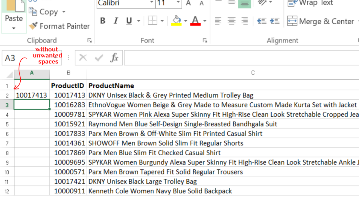
As you can see, the value in cell A2 is now closer to the line and without any leading space. The next few steps will guide you on how to replicate the result in the rest of the rows in column A2.
7. Select cell A2 (10017413),hover your cursur towards the the tiny square on the right side of the green triangle.
8. Double click to automatically fill the rest of the row so that your result will look like Fig. 8
Now that we have cleaned the unwanted spaces, we need to delete one of the columns since it is not right to have duplicates.
Follow the steps below to complete the process.
STEPS:9. Place your cursor on cell A2, press Ctrl Shift Down arrow key simultaneously to select the entire column.
10.Ctrl C to copy the values.
11.Ctrl Shift Up arrow key to go back up.
12.Select cell B2
13.Navigate to Paste in the Home Tab.
14. Click the drop down arrow and select 'value' under the paste values session.This will copy the values in column A into column B seamlessly.
See video 2 for a demo.
After this, right-click on column A and select delete.
PS:Don’t make the mistake of doing the normal copy-paste method because it won’t give you the expected result.
Manual line breaks and non-printing characters sometimes appear in a dataset. To get rid of this, use the CLEAN function. In some cases, the CLEAN and TRIM functions are used together, especially when the dataset is large and impossible to spot all the line breaks and extra characters.
For example, in this tutorial sample dataset, there appear not to be any visible line breaks, but it is advisable to use the CLEAN with the TRIM when dealing with unwanted spaces as discussed in number #2 above.
Refer to Video #3 for a demo on how to combine both functions.
To copy and paste the values, refer to steps 9–14 in #3
Having multiple entries in a dataset can affect the accuracy of your analysis as well as your model building. Therefore you need to deal with it. You either highlight it first or just delete it.
Delete Duplicate Data:
Excel allows you to define what duplicates are and also select the columns to remove the duplicates from.
STEPS:Select Data > Remove Duplicates > Check the data has header > check columns to remove duplicates from > Click OK
Make sure to check the box for header if your data has headers.
Missing values can have a significant effect on the result and invariably, the conclusions you draw from it. While there are different ways to deal with missing values, the most important thing is not to ignore them.
You can decide to fill the missing cells with ‘None’, ‘0’, or any other word. Use the steps below to highlight and fill the blank cells.
STEPS:1.Select the entire dataset.
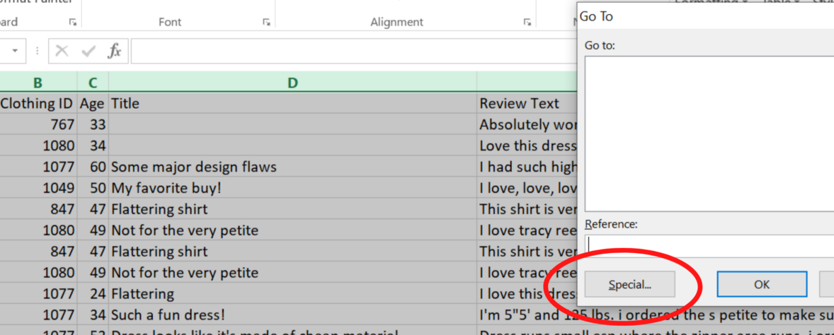
2.Hit the F5 key to open the 'Go To' dialogue box.
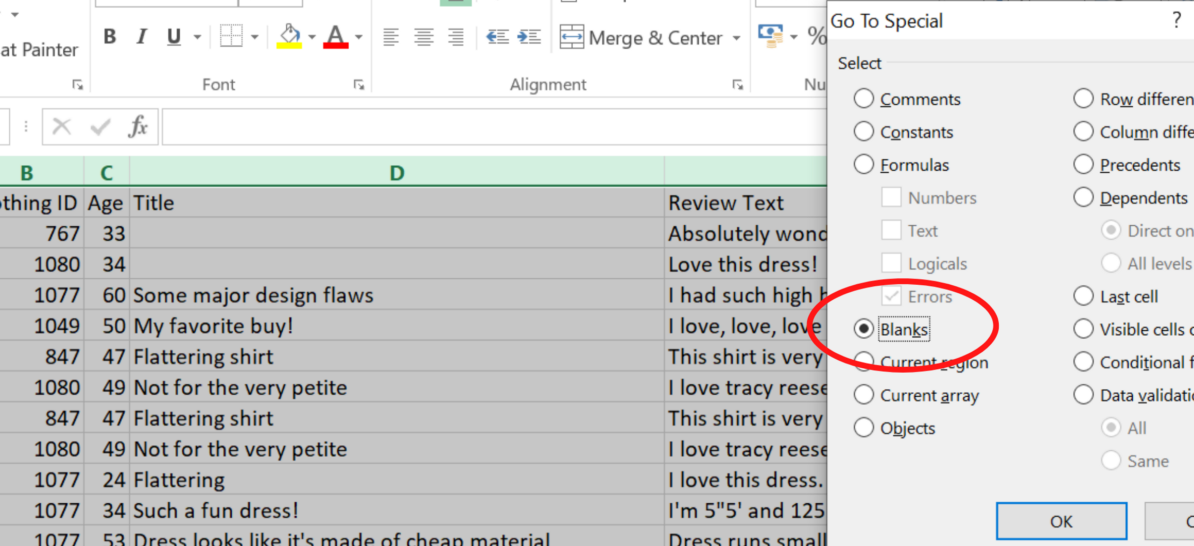
3.Click Special >select blank> click ok
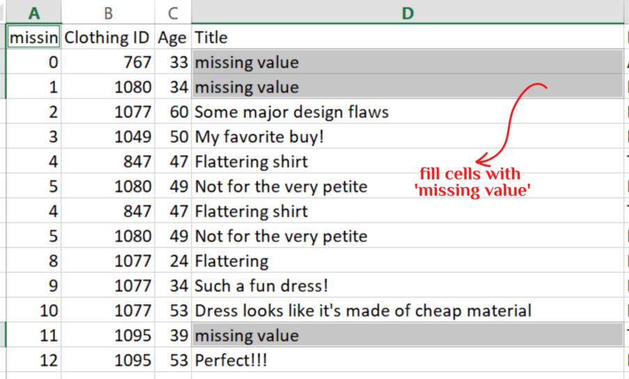
4.Type what you want to fillin the blank cells
5.Press CNTRL ENTER to automatically fill the word in all the blank cells.
PS:After typing, ‘missing value’, remember to press Ctrl ENTER. If you press ENTER alone, the word you typed will appear on just a single cell and the other blank cells will still remain blank.
Another common thing in working with the dataset is inconsistent sentence cases. For instance, a column might have a combination of upper, lower, and proper cases. You can use three Functions to convert the entire column to the most suitable sentence case.
=LOWER()— Converts all text into Lower Case.
=UPPER() — Converts all text into Upper Case.
=PROPER— Converts all Text into Proper Case.
STEPS:
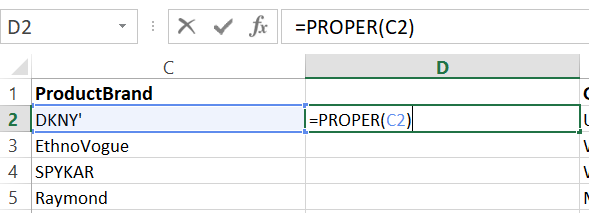
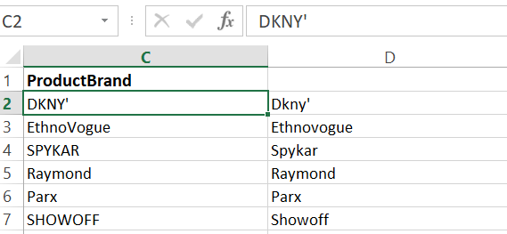
1.Create a new column next to the ProductBand.
2.Type =PROPER(C2)-Where C2 is the cell reference of 'DKNY' in column C.(Fig.15)
3.Press Enter and you should have 'DKNY' converted to 'Dkny'.
4.Follow the procedure in the video to replicate the result in the rest of the rows.
Again, we can’t have duplicate columns, so decide on the sentence case you prefer and refer to #2 on how to copy and paste values. Then delete the columns you don’t need.
Follow the steps used in =PROPER()to apply the =LOWER()and =UPPER()functions.Refer to video 6 for a demo of the three functions.
Great work for making it to the conclusion part. If you have any questions, feedback, or a special request, don’t hesitate to drop them in the comment session or reach out to me on LinkedIn. If you haven’t read the first article click HERE to start.
Also, these are just a few of the data cleaning techniques used in Excel. In the next tutorial, I will discuss 6 more and then do a full data cleaning project.
Sounds good?
See you soon!
Hope you enjoyed reading this article as much as I enjoyed writing it.
Don’t hesitate to drop your questions and contributions in the comment session.
Connect with me on LinkedIn.
CHEERS!
A comprehensive blueprint on getting started with data analysis in Microsoft Excel

Welcome to tutorial #2 of the Excel Series. Click HERE to read tutorial #1. Otherwise, proceed to tutorial #2 below.
The data cleaning techniques to cover in this tutorial are;
- Resize columns
- Get rid of leading and trailing spaces.
- Remove line breaks from cells
- Remove Duplicates
- Deal with blank rows and cells
- Standardize sentence case
The datasets used are fashion datasets from Kaggle and you can access them here>>> dataset 1 and dataset 2
Let’s get started!
Sometimes, when you import your dataset into Excel, some of the columns appear to be squashed making it difficult to see the entire values in each cell. An example is seen in Fig. 1 below.
There are different ways to resolve this but a faster approach would involve two steps.
STEPS:1.Select the 'all button'(to the left of column 'A').
2.Double click on any of the boundary lines between the columns.
This will automatically resize all columns as shown in Fig. 4.
The same data is shown in Fig. 4 but now looks more readable.
Leading and trailing spaces are unnecessary gaps that appear at the beginning, between, or end of data input and they might be difficult to spot. An example is shown in Column A, Fig. 5.
To get rid of these spaces, use the TRIM function.
Syntax:
=TRIM(text)
STEPS:1. Place your cursor on the column (ProductID) you wish to clean, hit Ctrl shift + at the same time.
2. Select'Entire column'as illustrated in Fig. 6a
3. Click ok.(This will create a new column to the left of ProductID).
4. In the new column(column A),Type =TRIM(B2);where B2 is the cell reference for ProductID. See Fig. 6b
5. Press ENTER
6. The result will be a cell with '1001743' and without the unwanted spaces as shown in Fig.7 and Video 2.
As you can see, the value in cell A2 is now closer to the line and without any leading space. The next few steps will guide you on how to replicate the result in the rest of the rows in column A2.
7. Select cell A2 (10017413),hover your cursur towards the the tiny square on the right side of the green triangle.
8. Double click to automatically fill the rest of the row so that your result will look like Fig. 8
Now that we have cleaned the unwanted spaces, we need to delete one of the columns since it is not right to have duplicates.
Follow the steps below to complete the process.
STEPS:9. Place your cursor on cell A2, press Ctrl Shift Down arrow key simultaneously to select the entire column.
10.Ctrl C to copy the values.
11.Ctrl Shift Up arrow key to go back up.
12.Select cell B2
13.Navigate to Paste in the Home Tab.
14. Click the drop down arrow and select 'value' under the paste values session.This will copy the values in column A into column B seamlessly.
See video 2 for a demo.
After this, right-click on column A and select delete.
PS:Don’t make the mistake of doing the normal copy-paste method because it won’t give you the expected result.
Manual line breaks and non-printing characters sometimes appear in a dataset. To get rid of this, use the CLEAN function. In some cases, the CLEAN and TRIM functions are used together, especially when the dataset is large and impossible to spot all the line breaks and extra characters.
For example, in this tutorial sample dataset, there appear not to be any visible line breaks, but it is advisable to use the CLEAN with the TRIM when dealing with unwanted spaces as discussed in number #2 above.
Refer to Video #3 for a demo on how to combine both functions.
To copy and paste the values, refer to steps 9–14 in #3
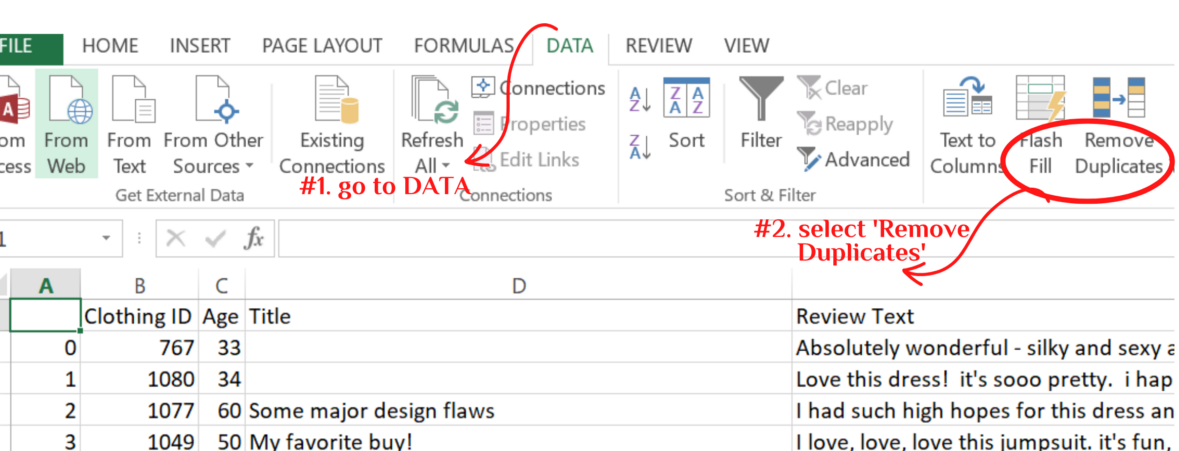
Having multiple entries in a dataset can affect the accuracy of your analysis as well as your model building. Therefore you need to deal with it. You either highlight it first or just delete it.
Delete Duplicate Data:
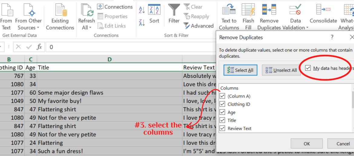
Excel allows you to define what duplicates are and also select the columns to remove the duplicates from.
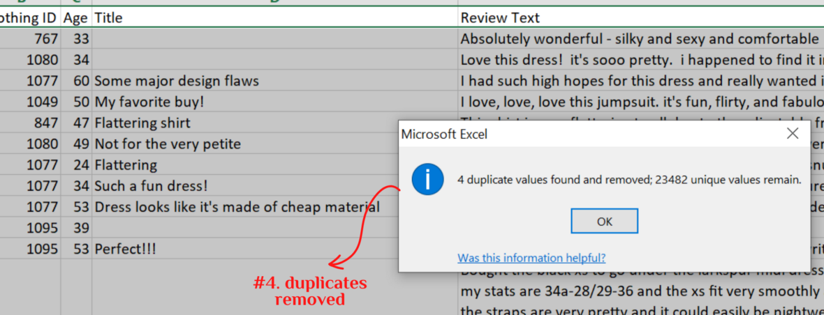
STEPS:Select Data > Remove Duplicates > Check the data has header > check columns to remove duplicates from > Click OK
Make sure to check the box for header if your data has headers.
Missing values can have a significant effect on the result and invariably, the conclusions you draw from it. While there are different ways to deal with missing values, the most important thing is not to ignore them.
You can decide to fill the missing cells with ‘None’, ‘0’, or any other word. Use the steps below to highlight and fill the blank cells.
STEPS:1.Select the entire dataset.
2.Hit the F5 key to open the 'Go To' dialogue box.
3.Click Special >select blank> click ok
4.Type what you want to fillin the blank cells
5.Press CNTRL ENTER to automatically fill the word in all the blank cells.
PS:After typing, ‘missing value’, remember to press Ctrl ENTER. If you press ENTER alone, the word you typed will appear on just a single cell and the other blank cells will still remain blank.
Another common thing in working with the dataset is inconsistent sentence cases. For instance, a column might have a combination of upper, lower, and proper cases. You can use three Functions to convert the entire column to the most suitable sentence case.
=LOWER()— Converts all text into Lower Case.
=UPPER() — Converts all text into Upper Case.
=PROPER— Converts all Text into Proper Case.
STEPS:
1.Create a new column next to the ProductBand.
2.Type =PROPER(C2)-Where C2 is the cell reference of 'DKNY' in column C.(Fig.15)
3.Press Enter and you should have 'DKNY' converted to 'Dkny'.
4.Follow the procedure in the video to replicate the result in the rest of the rows.
Again, we can’t have duplicate columns, so decide on the sentence case you prefer and refer to #2 on how to copy and paste values. Then delete the columns you don’t need.
Follow the steps used in =PROPER()to apply the =LOWER()and =UPPER()functions.Refer to video 6 for a demo of the three functions.
Great work for making it to the conclusion part. If you have any questions, feedback, or a special request, don’t hesitate to drop them in the comment session or reach out to me on LinkedIn. If you haven’t read the first article click HERE to start.
Also, these are just a few of the data cleaning techniques used in Excel. In the next tutorial, I will discuss 6 more and then do a full data cleaning project.
Sounds good?
See you soon!
Hope you enjoyed reading this article as much as I enjoyed writing it.
Don’t hesitate to drop your questions and contributions in the comment session.
Connect with me on LinkedIn.
CHEERS!
Denial of responsibility! Techno Blender is an automatic aggregator of the all world’s media. In each content, the hyperlink to the primary source is specified. All trademarks belong to their rightful owners, all materials to their authors. If you are the owner of the content and do not want us to publish your materials, please contact us by email – [email protected]. The content will be deleted within 24 hours.