
Data Drift Explainability: Interpretable Shift Detection with NannyML | by Marco Cerliani | Jun, 2022
Alerting Meaningful Multivariate Drift and ensuring Data Quality
Model monitoring is becoming a hot trend in machine learning. With the crescent hype in the activities concerning the MLOps, we register the rise of tools and research about the topic.
One of the most interesting is for sure the Confidence-based Performance Estimation (CBPE) algorithm developed by NannyML. They implemented a novel procedure to estimate future models’ performance degradation in absence of ground truth. It may yield great advantages in detecting performance drops since, in real applications, the labels could be expensive to collect and available in delay.
The CBPE algorithm is available in the NannyML package together with some interesting shift detection strategies. From the standard univariate drift detection methods to the more advanced multivariate feature drift approaches, we have at our disposal a great arsenal to automatically detect silent model failures.
In this post, we focus on the multivariate shit detection strategies. We want to investigate how to detect a multivariate feature shift. We make a comparison with the univariate case to demonstrate why the latter, in some cases, could not be enough to alert data drift. In the end, we make a step further, introducing a hybrid approach to provide explainable multivariate drift detection.
Univariate drift takes place when a variable registers a significant difference in distribution. Practically, we monitor each feature independently and check whether its distribution change over time. It could be carried out straightforwardly by comparing statistics between the new observations and past ones. For these reasons, univariate detection is easy to communicate and fully understandable.

Multivariate drift occurs when the relationships between input data change. Detecting multivariate changes could be more complicated to interpret, but often it is required to override the pitfalls of univariate detection.

The causes behind univariate and multivariate drift may vary according to use cases. Whatever the application, the results of univariate feature drift may be misleading. Let’s investigate why.
Supposing we have at our disposal four series of data (obtained through a simulation): two correlated sinusoids and two random noise features. We also consider two subsets (periods) of data to carry out our experiment. With the “reference” period we are referring to the historical data at our disposal. With the “analysis” period we are referring to the new samples we want to analyze.

In our “reference” period, the data follow the same patterns maintaining unchanged their relationship. In the “analysis” period we observe a variation in the verse of the relationship between the blue and the red sinusoids. More precisely, the two features are positively correlated in the “reference” period while they become negatively correlated by the end of the “analysis” period.


The relationship is changed but the univariate distributions remain unchanged. Can our univariate drift detection be effective?


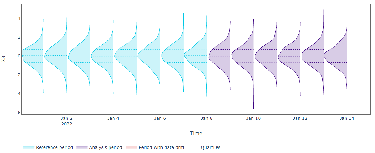

As expected, the univariate data drift detection algorithms don’t reveal any drift for all the features under analysis. From the plots above, we can see that univariate distributions don’t change over time so the Kolmogorov–Smirnov test can’t alert shift. We need a more effective approach.
Everyone, who attended a basic machine learning course, has already encountered the Principal Component Analysis (PCA). It’s a technique to carry out dimensionality reduction of tabular datasets preserving the most salient interactions. At the same time, we can use the PCA to reverse the compressed data to their original shape. This reconstruction procedure can preserve only the meaningful patterns in the data while discharging the noise.

NannyML leverages the reconstruction ability of the PCA to develop a simple and effective method for multivariate drift detection.
A set of data is firstly compressed into a lower dimensionality space and, secondly, decompressed to return to the original feature dimensionality. This transformation process is the key to reconstructing our data preserving only the relevant interactions. At this point, it’s possible to compute the series of reconstruction errors (as simple Euclidean distance) between the original data and the transformed counterpart. Any meaningful spike from the series of the reconstruction errors can be viewed as a change in the data relationship, aka multivariate drift.
Let’s see this methodology in action on our data.
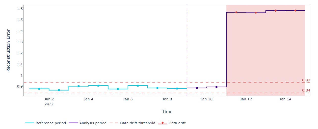
We fit the PCA on our “reference” dataset and compute the reconstruction errors. This is useful to establish the upper and lower bounds used to detect changes in the future “analysis” data. When new data becomes available, we only have to compress and reconstruct them using the fitted PCA. If the reconstruction errors fall outside the expected thresholds we should register a change in feature relationships. That is exactly what happened with our data.
The PCA methodology gives useful insights for multivariate drift detection. With a single KPI, we could control the entire system status. At the same time, disjointing the contribution of each feature may be added value.
With the PCA we aim to learn patterns in a single learning step. That’s great and reveals to be effective in most cases and in several applications. If our goal is to discover the unknown relationships between features, we could do the same in a straightforward way.
We could imagine the relationship discovery as a supervised task. In other words, given a set of features, we could use them to predict each other and use the generated residuals as a measure of drift. If the residuals vary with the passing of time, we notify a shift.

Coming back to our simulated scenario, we fit one model for each feature at our disposal on the “reference” data. Each model is fitted to predict the desired feature using all the other features as predictors. Then we generated the residuals both on “reference” and “analysis” data. Having at disposal series of residuals we could detect drift using univariate approaches.


Detecting drift with univariate methodologies is now more effective. We register high errors at the end of the “analysis” period for both X1 and X2. More precisely, we have no evidence of a univariate distribution drift for X1 and X2 in the same period. For this reason, the high errors may indicate a change in the relationship between X1 and the rest of the input data (the same for X2). In other words, the shift in univariate reconstruction error distributions may reveal that the involved features have changed their interactions.
In this post, we introduced some recent techniques available for effective data drift monitoring. We also understood how and why only a univariate approach could suffer. We discovered the importance of multivariate feature shift and tried to provide an explainable method to identify the sources of possible multivariate drift.
Alerting Meaningful Multivariate Drift and ensuring Data Quality
Model monitoring is becoming a hot trend in machine learning. With the crescent hype in the activities concerning the MLOps, we register the rise of tools and research about the topic.
One of the most interesting is for sure the Confidence-based Performance Estimation (CBPE) algorithm developed by NannyML. They implemented a novel procedure to estimate future models’ performance degradation in absence of ground truth. It may yield great advantages in detecting performance drops since, in real applications, the labels could be expensive to collect and available in delay.
The CBPE algorithm is available in the NannyML package together with some interesting shift detection strategies. From the standard univariate drift detection methods to the more advanced multivariate feature drift approaches, we have at our disposal a great arsenal to automatically detect silent model failures.
In this post, we focus on the multivariate shit detection strategies. We want to investigate how to detect a multivariate feature shift. We make a comparison with the univariate case to demonstrate why the latter, in some cases, could not be enough to alert data drift. In the end, we make a step further, introducing a hybrid approach to provide explainable multivariate drift detection.
Univariate drift takes place when a variable registers a significant difference in distribution. Practically, we monitor each feature independently and check whether its distribution change over time. It could be carried out straightforwardly by comparing statistics between the new observations and past ones. For these reasons, univariate detection is easy to communicate and fully understandable.
Multivariate drift occurs when the relationships between input data change. Detecting multivariate changes could be more complicated to interpret, but often it is required to override the pitfalls of univariate detection.
The causes behind univariate and multivariate drift may vary according to use cases. Whatever the application, the results of univariate feature drift may be misleading. Let’s investigate why.
Supposing we have at our disposal four series of data (obtained through a simulation): two correlated sinusoids and two random noise features. We also consider two subsets (periods) of data to carry out our experiment. With the “reference” period we are referring to the historical data at our disposal. With the “analysis” period we are referring to the new samples we want to analyze.
In our “reference” period, the data follow the same patterns maintaining unchanged their relationship. In the “analysis” period we observe a variation in the verse of the relationship between the blue and the red sinusoids. More precisely, the two features are positively correlated in the “reference” period while they become negatively correlated by the end of the “analysis” period.
The relationship is changed but the univariate distributions remain unchanged. Can our univariate drift detection be effective?
As expected, the univariate data drift detection algorithms don’t reveal any drift for all the features under analysis. From the plots above, we can see that univariate distributions don’t change over time so the Kolmogorov–Smirnov test can’t alert shift. We need a more effective approach.
Everyone, who attended a basic machine learning course, has already encountered the Principal Component Analysis (PCA). It’s a technique to carry out dimensionality reduction of tabular datasets preserving the most salient interactions. At the same time, we can use the PCA to reverse the compressed data to their original shape. This reconstruction procedure can preserve only the meaningful patterns in the data while discharging the noise.
NannyML leverages the reconstruction ability of the PCA to develop a simple and effective method for multivariate drift detection.
A set of data is firstly compressed into a lower dimensionality space and, secondly, decompressed to return to the original feature dimensionality. This transformation process is the key to reconstructing our data preserving only the relevant interactions. At this point, it’s possible to compute the series of reconstruction errors (as simple Euclidean distance) between the original data and the transformed counterpart. Any meaningful spike from the series of the reconstruction errors can be viewed as a change in the data relationship, aka multivariate drift.
Let’s see this methodology in action on our data.
We fit the PCA on our “reference” dataset and compute the reconstruction errors. This is useful to establish the upper and lower bounds used to detect changes in the future “analysis” data. When new data becomes available, we only have to compress and reconstruct them using the fitted PCA. If the reconstruction errors fall outside the expected thresholds we should register a change in feature relationships. That is exactly what happened with our data.
The PCA methodology gives useful insights for multivariate drift detection. With a single KPI, we could control the entire system status. At the same time, disjointing the contribution of each feature may be added value.
With the PCA we aim to learn patterns in a single learning step. That’s great and reveals to be effective in most cases and in several applications. If our goal is to discover the unknown relationships between features, we could do the same in a straightforward way.
We could imagine the relationship discovery as a supervised task. In other words, given a set of features, we could use them to predict each other and use the generated residuals as a measure of drift. If the residuals vary with the passing of time, we notify a shift.
Coming back to our simulated scenario, we fit one model for each feature at our disposal on the “reference” data. Each model is fitted to predict the desired feature using all the other features as predictors. Then we generated the residuals both on “reference” and “analysis” data. Having at disposal series of residuals we could detect drift using univariate approaches.
Detecting drift with univariate methodologies is now more effective. We register high errors at the end of the “analysis” period for both X1 and X2. More precisely, we have no evidence of a univariate distribution drift for X1 and X2 in the same period. For this reason, the high errors may indicate a change in the relationship between X1 and the rest of the input data (the same for X2). In other words, the shift in univariate reconstruction error distributions may reveal that the involved features have changed their interactions.
In this post, we introduced some recent techniques available for effective data drift monitoring. We also understood how and why only a univariate approach could suffer. We discovered the importance of multivariate feature shift and tried to provide an explainable method to identify the sources of possible multivariate drift.
Denial of responsibility! Techno Blender is an automatic aggregator of the all world’s media. In each content, the hyperlink to the primary source is specified. All trademarks belong to their rightful owners, all materials to their authors. If you are the owner of the content and do not want us to publish your materials, please contact us by email – [email protected]. The content will be deleted within 24 hours.