
Decision Trees, Explained. How to train them and how they work… | by Uri Almog | May, 2022
How to train them and how they work, with working code examples
In this post we’re going to discuss a commonly used machine learning model called decision tree. Decision trees are preferred for many applications, mainly due to their high explainability, but also due to the fact that they are relatively simple to set up and train, and the short time it takes to perform a prediction with a decision tree. Decision trees are natural to tabular data, and, in fact, they currently seem to outperform neural networks on that type of data (as opposed to images). Unlike neural networks, trees don’t require input normalization, since their training is not based on gradient descent and they have very few parameters to optimize on. They can even train on data with missing values, but nowadays this practice is less recommended, and missing values are usually imputed.
Among the well-known use-cases for decision trees are recommendation systems (what are your predicted movie preferences based on your past choices and other features, e.g. age, gender etc.) and search engines.
The prediction process in a tree is composed of a sequence of comparisons of the sample’s attributes (features) with pre-learned threshold values. Starting from the top (the root of the tree) and going downward (toward the leaves, yes, opposite to real-life trees), in each step the result of the comparison determines if the sample goes left or right in the tree, and by that — determines the next comparison step. When our sample reaches a leaf (an end node) — the decision, or prediction, is made, based on the majority class in the leaf.
Fig.1 shows this process with a problem of classifying Iris samples into 3 different species (classes) based on their petal and sepal lengths and widths.
Our example will be based on the famous Iris dataset (Fisher, R.A. “The use of multiple measurements in taxonomic problems” Annual Eugenics, 7, Part II, 179–188 (1936)). I downloaded it using sklearn package, which is a BSD (Berkley Source Distribution) license software. I modified the features of one of the classes and decreased the train set size, to mix the classes a little bit and make it more interesting.

We’ll work out the details of this tree later. For now, we’ll examine the root node and notice that our training population has 45 samples, divided into 3 classes like so: [13, 19, 13]. The ‘class’ attribute tells us the label the tree would predict for this sample if it were a leaf — based on the majority class in the node. For example — if we weren’t allowed to run any comparisons, we would be in the root node and our best prediction would be class Veriscolor, since it has 19 samples in the train set, vs. 13 for the other two classes. If our sequence of comparisons led us to the leaf second from left, the model’s prediction would, again, be Veriscolor, since in the training set there were 4 samples of that class that reached this leaf, vs. only 1 sample of class Virginica and zero samples of class Setosa.
Decision trees can be used for either classification or regression problems. Let’s start by discussing the classification problem and explain how the tree training algorithm works.
Let’s see how we train a tree using sklearn and then discuss the mechanism.
Downloading the dataset:
import numpy as np
from sklearn.datasets import load_iris
from sklearn.model_selection import train_test_split
from sklearn.preprocessing import OneHotEncoderiris = load_iris()
X = iris['data']
y = iris['target']
names = iris['target_names']
feature_names = iris['feature_names']# One hot encoding
enc = OneHotEncoder()
Y = enc.fit_transform(y[:, np.newaxis]).toarray()# Modifying the dataset
X[y==1,2] = X[y==1,2] + 0.3# Split the data set into training and testing
X_train, X_test, Y_train, Y_test = train_test_split(
X, Y, test_size=0.5, random_state=2)# Decreasing the train set to make things more interesting
X_train = X_train[30:,:]
Y_train = Y_train[30:,:]
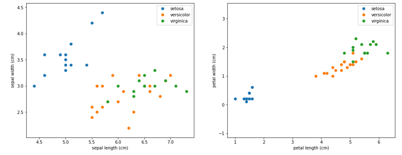
Let’s visualize the dataset.
# Visualize the data sets
import matplotlib
import matplotlib.pyplot as pltplt.figure(figsize=(16, 6))
plt.subplot(1, 2, 1)
for target, target_name in enumerate(names):
X_plot = X[y == target]
plt.plot(X_plot[:, 0], X_plot[:, 1], linestyle='none', marker='o', label=target_name)
plt.xlabel(feature_names[0])
plt.ylabel(feature_names[1])
plt.axis('equal')
plt.legend();plt.subplot(1, 2, 2)
for target, target_name in enumerate(names):
X_plot = X[y == target]
plt.plot(X_plot[:, 2], X_plot[:, 3], linestyle='none', marker='o', label=target_name)
plt.xlabel(feature_names[2])
plt.ylabel(feature_names[3])
plt.axis('equal')
plt.legend();

and just the train set:
plt.figure(figsize=(16, 6))
plt.subplot(1, 2, 1)
for target, target_name in enumerate(names):
X_plot = X_train[Y_train[:,target] == 1]
plt.plot(X_plot[:, 0], X_plot[:, 1], linestyle='none', marker='o', label=target_name)
plt.xlabel(feature_names[0])
plt.ylabel(feature_names[1])
plt.axis('equal')
plt.legend();plt.subplot(1, 2, 2)
for target, target_name in enumerate(names):
X_plot = X_train[Y_train[:,target] == 1]
plt.plot(X_plot[:, 2], X_plot[:, 3], linestyle='none', marker='o', label=target_name)
plt.xlabel(feature_names[2])
plt.ylabel(feature_names[3])
plt.axis('equal')
plt.legend();
Now we are ready to train a tree and visualize it. The result is the model that we saw in Fig.1.
from sklearn import tree
import graphviziristree = tree.DecisionTreeClassifier(max_depth=3, criterion='gini', random_state=0)
iristree.fit(X_train, enc.inverse_transform(Y_train))feature_names = ['sepal length', 'sepal width', 'petal length', 'petal width']dot_data = tree.export_graphviz(iristree, out_file=None,
feature_names=feature_names,
class_names=names,
filled=True, rounded=True,
special_characters=True)
graph = graphviz.Source(dot_data)display(graph)
We can see that the tree uses the petal width for its first and second splits — the first split cleanly separates class Setosa from the other two. Note that for the first split, the petal length could work equally well.
Let’s see the classification precision of this model on the train set, followed by the test set:
from sklearn.metrics import precision_score
from sklearn.metrics import recall_scoreiristrainpred = iristree.predict(X_train)
iristestpred = iristree.predict(X_test)# train precision:
display(precision_score(enc.inverse_transform(Y_train), iristrainpred.reshape(-1,1), average='micro', labels=[0]))
display(precision_score(enc.inverse_transform(Y_train), iristrainpred.reshape(-1,1), average='micro', labels=[1]))
display(precision_score(enc.inverse_transform(Y_train), iristrainpred.reshape(-1,1), average='micro', labels=[2]))>>> 1.0
>>> 0.9047619047619048
>>> 1.0# test precision:
display(precision_score(enc.inverse_transform(Y_test), iristestpred.reshape(-1,1), average='micro', labels=[0]))
display(precision_score(enc.inverse_transform(Y_test), iristestpred.reshape(-1,1), average='micro', labels=[1]))
display(precision_score(enc.inverse_transform(Y_test), iristestpred.reshape(-1,1), average='micro', labels=[2]))>>> 1.0
>>> 0.7586206896551724
>>> 0.9473684210526315
As we can see, the scarcity of data in our training set and the fact that classes 1 and 2 are mixed (because we modified the dataset) resulted in a lower precision on those classes in the test set. Class 0 maintains perfect precision because it is highly separated from the other two.
In other words — how does it choose the optimal features and thresholds to put in each node?
Gini Impurity
As in other machine learning models, a decision tree training mechanism tries to minimize some loss caused by prediction error on the train set. The Gini impurity index (after the Italian statistician Corrado Gini) is a natural measure for classification accuracy.
A high Gini corresponds to a heterogeneous population (similar sample amounts from each class) while a low Gini indicates a homogeneous population (i.e. it is composed mainly of a single class)
The maximum possible Gini value depends on the number of classes: in a classification problem with C classes, the maximum possible Gini is 1–1/C (when the classes are evenly populated). The minimum Gini is 0 and it is achieved when the entire population is composed of a single class.
The Gini impurity index is the expectation value of wrong classifications if the classification is done in random.
Why?
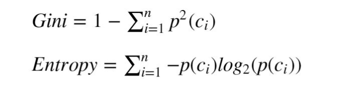
Because the probability to randomly pick a sample from class ci is p(ci). Having picked that, the probability to predict the wrong class is (1-p(ci)). If we sum p(ci)*(1-p(ci)) over all the classes we get the formula for the Gini impurity in Fig.4.
With the Gini index as objective, the tree chooses in each step the feature and threshold that split the population in a way that maximally decreases the weighted average Gini of the two resulting populations (or maximally increase their weighted average homogeneity). In other words, the train logic is to minimize the probability of random classification error in the two resulting populations, with more weight put on the larger of the sub populations.
And yes — the mechanism goes over all the sample values and splits them according to the criterion to check the resulting Gini.
From this definition we can also understand why the threshold values are always actual values found on at least one of the train samples — there is no gain in using a value that is in the gap between samples since the resulting split would be identical.
Another metric that is commonly used for tree training is entropy (see formula in Fig.4).
Entropy
While the Gini strategy aims to minimize the random classification error in the next step, the entropy minimization strategy aims to maximize the information gain.
Information gain
In absence of a prior knowledge of how a population is divided into 10 classes, we assume it’s divided evenly between them. In this case, we need an average of 3.3 yes/no questions to find out the classification of a sample (are you class 1–5? If not — are you class 6–8? etc.). This means that the entropy of the population is 3.3 bits.
but now let’s assume that we did something (like a clever split) that gave us information on the population distribution, and now we know that 50% of the samples are in class 1, 25% in class 2 and 25% of the samples in class 3. In this case the entropy of the population will be 1.5 — we only need 1.5 bits to describe a random sample. (First question — are you class 1? The sequence will end here 50% of the time. Second question — are you class 2? and no more questions are required — so 50%*1 + 50%*2 = 1.5 questions on average). That information we gained is worth 1.8 bits.
Like Gini, minimizing entropy is also aligned with creating a more homogeneous population, since homogeneous populations have lower entropy (with the extreme of a single-class population having a 0 entropy — no need to ask any yes/no questions).
Gini or Entropy?
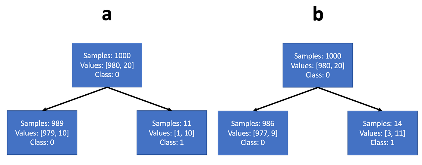
Most sources claim that the difference between the two strategies is not that significant (indeed — if you try to train an entropy tree on the problem we just worked — you will get exactly the same splits). It’s easy to see why: while Gini maximizes the expectation value of a class probability, entropy maximizes the expectation value of the log class probability. But the log probability is a monotonically increasing function of the probability, so they usually operate quite similarly. However, entropy minimization may choose a different configuration than Gini, when the population is highly unbalanced. For example, we can think of a dataset with 1000 training samples — 980 belong to class 0 and 20 to class 1. Let’s say the tree can choose a threshold that would split it either according to example a or example b in Fig.5. We note that both examples create a node with a large population composed mainly of the majority class, and the a second node with small population composed mainly of the minority class.
In such a case, the steepness of the log function at small values will motivate the entropy criterion to purify the node with the large population, more strongly than the Gini criterion. So if we work out the math, we’ll see that the Gini criterion would choose split a, and the entropy criterion would chooses split b.
This may lead to a different choice of feature/threshold. Not necessarily better or worse — this depends on our goals.
Note that even in problems with initially balanced populations, the lower nodes of the classification tree will typically have highly unbalanced populations.
When a path in the tree reaches the specified depth value, or when it contains a zero Gini/entropy population, it stops training. When all the paths stopped training, the tree is ready.
A common practice is to limit the depth of a tree. Another is to limit the number of samples in a leaf (not allowing fewer samples than a threshold). Both practices are done to prevent overfitting on the train set.
Now that we’ve worked out the details on training a classification tree, it will be very straightforward to understand regression trees: The labels in regression problems are continuous rather than discrete (e.g. the effectiveness of a given drug dose, measured in % of the cases). Training on this type of problem, regression trees also classify, but the labels are dynamically calculated as the mean value of the samples in each node. Here, it is common to use mean square error or Chi square measure as objectives for minimization, instead of Gini and entropy.
In this post we learned that decision trees are basically comparison sequences that can train to perform classification and regression tasks. We ran python scripts that trained a decision tree classifier, used our classifier to predict the class of several data samples, and computed the precision and recall metrics of the predictions on the training set and the test set. We also learned the mathematical mechanism behind the decision tree training, that aims to minimize some prediction error metric (Gini, entropy, mse) after each comparison. I hope you enjoyed reading this post, see you in my other posts!
How to train them and how they work, with working code examples

In this post we’re going to discuss a commonly used machine learning model called decision tree. Decision trees are preferred for many applications, mainly due to their high explainability, but also due to the fact that they are relatively simple to set up and train, and the short time it takes to perform a prediction with a decision tree. Decision trees are natural to tabular data, and, in fact, they currently seem to outperform neural networks on that type of data (as opposed to images). Unlike neural networks, trees don’t require input normalization, since their training is not based on gradient descent and they have very few parameters to optimize on. They can even train on data with missing values, but nowadays this practice is less recommended, and missing values are usually imputed.
Among the well-known use-cases for decision trees are recommendation systems (what are your predicted movie preferences based on your past choices and other features, e.g. age, gender etc.) and search engines.
The prediction process in a tree is composed of a sequence of comparisons of the sample’s attributes (features) with pre-learned threshold values. Starting from the top (the root of the tree) and going downward (toward the leaves, yes, opposite to real-life trees), in each step the result of the comparison determines if the sample goes left or right in the tree, and by that — determines the next comparison step. When our sample reaches a leaf (an end node) — the decision, or prediction, is made, based on the majority class in the leaf.
Fig.1 shows this process with a problem of classifying Iris samples into 3 different species (classes) based on their petal and sepal lengths and widths.
Our example will be based on the famous Iris dataset (Fisher, R.A. “The use of multiple measurements in taxonomic problems” Annual Eugenics, 7, Part II, 179–188 (1936)). I downloaded it using sklearn package, which is a BSD (Berkley Source Distribution) license software. I modified the features of one of the classes and decreased the train set size, to mix the classes a little bit and make it more interesting.
We’ll work out the details of this tree later. For now, we’ll examine the root node and notice that our training population has 45 samples, divided into 3 classes like so: [13, 19, 13]. The ‘class’ attribute tells us the label the tree would predict for this sample if it were a leaf — based on the majority class in the node. For example — if we weren’t allowed to run any comparisons, we would be in the root node and our best prediction would be class Veriscolor, since it has 19 samples in the train set, vs. 13 for the other two classes. If our sequence of comparisons led us to the leaf second from left, the model’s prediction would, again, be Veriscolor, since in the training set there were 4 samples of that class that reached this leaf, vs. only 1 sample of class Virginica and zero samples of class Setosa.
Decision trees can be used for either classification or regression problems. Let’s start by discussing the classification problem and explain how the tree training algorithm works.
Let’s see how we train a tree using sklearn and then discuss the mechanism.
Downloading the dataset:
import numpy as np
from sklearn.datasets import load_iris
from sklearn.model_selection import train_test_split
from sklearn.preprocessing import OneHotEncoderiris = load_iris()
X = iris['data']
y = iris['target']
names = iris['target_names']
feature_names = iris['feature_names']# One hot encoding
enc = OneHotEncoder()
Y = enc.fit_transform(y[:, np.newaxis]).toarray()# Modifying the dataset
X[y==1,2] = X[y==1,2] + 0.3# Split the data set into training and testing
X_train, X_test, Y_train, Y_test = train_test_split(
X, Y, test_size=0.5, random_state=2)# Decreasing the train set to make things more interesting
X_train = X_train[30:,:]
Y_train = Y_train[30:,:]
Let’s visualize the dataset.
# Visualize the data sets
import matplotlib
import matplotlib.pyplot as pltplt.figure(figsize=(16, 6))
plt.subplot(1, 2, 1)
for target, target_name in enumerate(names):
X_plot = X[y == target]
plt.plot(X_plot[:, 0], X_plot[:, 1], linestyle='none', marker='o', label=target_name)
plt.xlabel(feature_names[0])
plt.ylabel(feature_names[1])
plt.axis('equal')
plt.legend();plt.subplot(1, 2, 2)
for target, target_name in enumerate(names):
X_plot = X[y == target]
plt.plot(X_plot[:, 2], X_plot[:, 3], linestyle='none', marker='o', label=target_name)
plt.xlabel(feature_names[2])
plt.ylabel(feature_names[3])
plt.axis('equal')
plt.legend();
and just the train set:
plt.figure(figsize=(16, 6))
plt.subplot(1, 2, 1)
for target, target_name in enumerate(names):
X_plot = X_train[Y_train[:,target] == 1]
plt.plot(X_plot[:, 0], X_plot[:, 1], linestyle='none', marker='o', label=target_name)
plt.xlabel(feature_names[0])
plt.ylabel(feature_names[1])
plt.axis('equal')
plt.legend();plt.subplot(1, 2, 2)
for target, target_name in enumerate(names):
X_plot = X_train[Y_train[:,target] == 1]
plt.plot(X_plot[:, 2], X_plot[:, 3], linestyle='none', marker='o', label=target_name)
plt.xlabel(feature_names[2])
plt.ylabel(feature_names[3])
plt.axis('equal')
plt.legend();
Now we are ready to train a tree and visualize it. The result is the model that we saw in Fig.1.
from sklearn import tree
import graphviziristree = tree.DecisionTreeClassifier(max_depth=3, criterion='gini', random_state=0)
iristree.fit(X_train, enc.inverse_transform(Y_train))feature_names = ['sepal length', 'sepal width', 'petal length', 'petal width']dot_data = tree.export_graphviz(iristree, out_file=None,
feature_names=feature_names,
class_names=names,
filled=True, rounded=True,
special_characters=True)
graph = graphviz.Source(dot_data)display(graph)
We can see that the tree uses the petal width for its first and second splits — the first split cleanly separates class Setosa from the other two. Note that for the first split, the petal length could work equally well.
Let’s see the classification precision of this model on the train set, followed by the test set:
from sklearn.metrics import precision_score
from sklearn.metrics import recall_scoreiristrainpred = iristree.predict(X_train)
iristestpred = iristree.predict(X_test)# train precision:
display(precision_score(enc.inverse_transform(Y_train), iristrainpred.reshape(-1,1), average='micro', labels=[0]))
display(precision_score(enc.inverse_transform(Y_train), iristrainpred.reshape(-1,1), average='micro', labels=[1]))
display(precision_score(enc.inverse_transform(Y_train), iristrainpred.reshape(-1,1), average='micro', labels=[2]))>>> 1.0
>>> 0.9047619047619048
>>> 1.0# test precision:
display(precision_score(enc.inverse_transform(Y_test), iristestpred.reshape(-1,1), average='micro', labels=[0]))
display(precision_score(enc.inverse_transform(Y_test), iristestpred.reshape(-1,1), average='micro', labels=[1]))
display(precision_score(enc.inverse_transform(Y_test), iristestpred.reshape(-1,1), average='micro', labels=[2]))>>> 1.0
>>> 0.7586206896551724
>>> 0.9473684210526315
As we can see, the scarcity of data in our training set and the fact that classes 1 and 2 are mixed (because we modified the dataset) resulted in a lower precision on those classes in the test set. Class 0 maintains perfect precision because it is highly separated from the other two.
In other words — how does it choose the optimal features and thresholds to put in each node?
Gini Impurity
As in other machine learning models, a decision tree training mechanism tries to minimize some loss caused by prediction error on the train set. The Gini impurity index (after the Italian statistician Corrado Gini) is a natural measure for classification accuracy.
A high Gini corresponds to a heterogeneous population (similar sample amounts from each class) while a low Gini indicates a homogeneous population (i.e. it is composed mainly of a single class)
The maximum possible Gini value depends on the number of classes: in a classification problem with C classes, the maximum possible Gini is 1–1/C (when the classes are evenly populated). The minimum Gini is 0 and it is achieved when the entire population is composed of a single class.
The Gini impurity index is the expectation value of wrong classifications if the classification is done in random.
Why?
Because the probability to randomly pick a sample from class ci is p(ci). Having picked that, the probability to predict the wrong class is (1-p(ci)). If we sum p(ci)*(1-p(ci)) over all the classes we get the formula for the Gini impurity in Fig.4.
With the Gini index as objective, the tree chooses in each step the feature and threshold that split the population in a way that maximally decreases the weighted average Gini of the two resulting populations (or maximally increase their weighted average homogeneity). In other words, the train logic is to minimize the probability of random classification error in the two resulting populations, with more weight put on the larger of the sub populations.
And yes — the mechanism goes over all the sample values and splits them according to the criterion to check the resulting Gini.
From this definition we can also understand why the threshold values are always actual values found on at least one of the train samples — there is no gain in using a value that is in the gap between samples since the resulting split would be identical.
Another metric that is commonly used for tree training is entropy (see formula in Fig.4).
Entropy
While the Gini strategy aims to minimize the random classification error in the next step, the entropy minimization strategy aims to maximize the information gain.
Information gain
In absence of a prior knowledge of how a population is divided into 10 classes, we assume it’s divided evenly between them. In this case, we need an average of 3.3 yes/no questions to find out the classification of a sample (are you class 1–5? If not — are you class 6–8? etc.). This means that the entropy of the population is 3.3 bits.
but now let’s assume that we did something (like a clever split) that gave us information on the population distribution, and now we know that 50% of the samples are in class 1, 25% in class 2 and 25% of the samples in class 3. In this case the entropy of the population will be 1.5 — we only need 1.5 bits to describe a random sample. (First question — are you class 1? The sequence will end here 50% of the time. Second question — are you class 2? and no more questions are required — so 50%*1 + 50%*2 = 1.5 questions on average). That information we gained is worth 1.8 bits.
Like Gini, minimizing entropy is also aligned with creating a more homogeneous population, since homogeneous populations have lower entropy (with the extreme of a single-class population having a 0 entropy — no need to ask any yes/no questions).
Gini or Entropy?
Most sources claim that the difference between the two strategies is not that significant (indeed — if you try to train an entropy tree on the problem we just worked — you will get exactly the same splits). It’s easy to see why: while Gini maximizes the expectation value of a class probability, entropy maximizes the expectation value of the log class probability. But the log probability is a monotonically increasing function of the probability, so they usually operate quite similarly. However, entropy minimization may choose a different configuration than Gini, when the population is highly unbalanced. For example, we can think of a dataset with 1000 training samples — 980 belong to class 0 and 20 to class 1. Let’s say the tree can choose a threshold that would split it either according to example a or example b in Fig.5. We note that both examples create a node with a large population composed mainly of the majority class, and the a second node with small population composed mainly of the minority class.
In such a case, the steepness of the log function at small values will motivate the entropy criterion to purify the node with the large population, more strongly than the Gini criterion. So if we work out the math, we’ll see that the Gini criterion would choose split a, and the entropy criterion would chooses split b.
This may lead to a different choice of feature/threshold. Not necessarily better or worse — this depends on our goals.
Note that even in problems with initially balanced populations, the lower nodes of the classification tree will typically have highly unbalanced populations.
When a path in the tree reaches the specified depth value, or when it contains a zero Gini/entropy population, it stops training. When all the paths stopped training, the tree is ready.
A common practice is to limit the depth of a tree. Another is to limit the number of samples in a leaf (not allowing fewer samples than a threshold). Both practices are done to prevent overfitting on the train set.
Now that we’ve worked out the details on training a classification tree, it will be very straightforward to understand regression trees: The labels in regression problems are continuous rather than discrete (e.g. the effectiveness of a given drug dose, measured in % of the cases). Training on this type of problem, regression trees also classify, but the labels are dynamically calculated as the mean value of the samples in each node. Here, it is common to use mean square error or Chi square measure as objectives for minimization, instead of Gini and entropy.
In this post we learned that decision trees are basically comparison sequences that can train to perform classification and regression tasks. We ran python scripts that trained a decision tree classifier, used our classifier to predict the class of several data samples, and computed the precision and recall metrics of the predictions on the training set and the test set. We also learned the mathematical mechanism behind the decision tree training, that aims to minimize some prediction error metric (Gini, entropy, mse) after each comparison. I hope you enjoyed reading this post, see you in my other posts!
Denial of responsibility! Techno Blender is an automatic aggregator of the all world’s media. In each content, the hyperlink to the primary source is specified. All trademarks belong to their rightful owners, all materials to their authors. If you are the owner of the content and do not want us to publish your materials, please contact us by email – [email protected]. The content will be deleted within 24 hours.