Deep Dive into Vector Databases by Hand ✍︎

Explore what exactly happens behind-the-scenes in Vector Databases

The other day I asked my favorite Large Language Model (LLM) to help me explain vectors to my almost 4-year old. In seconds, it spit out a story filled with mythical creatures and magic and vectors. And Voila! I had a sketch for a new children’s book, and it was impressive because the unicorn was called ‘LuminaVec’.

So, how did the model help weave this creative magic? Well, the answer is by using vectors (in real life) and most probably vector databases. How so? Let me explain.

Vectors and Embedding

First, the model doesn’t understand the exact words I typed in. What helps it understand the words are their numerical representations which are in the form of vectors. These vectors help the model find similarity among the different words while focusing on meaningful information about each. It does this by using embeddings which are low-dimensional vectors that try to capture the semantics and context of the information.

In other words, vectors in an embedding are lists of numbers that specify the position of an object with respect to a reference space. These objects can be features that define a variable in a dataset. With the help of these numerical vector values, we can determine how close or how far one feature is from the other — are they similar (close) or not similar (far)?

Now these vectors are quite powerful but when we are talking about LLMs, we need to be extra cautious about them because of the word ‘large’. As it happens to be with these ‘large’ models, these vectors may quickly become long and more complex, spanning over hundreds or even thousands of dimensions. If not dealt with carefully, the processing speed and mounting expense could become cumbersome very fast!

Vector Databases

To address this issue, we have our mighty warrior : Vector databases.

Vector databases are special databases that contain these vector embeddings. Similar objects have vectors that are closer to each other in the vector database, while dissimilar objects have vectors that are farther apart. So, rather than parsing the data every time a query comes in and generating these vector embeddings, which induces huge resources, it is much faster to run the data through the model once, store it in the vector database and retrieve it as needed. This makes vector databases one of the most powerful solutions addressing the problem of scale and speed for these LLMs.

So, going back to the story about the rainbow unicorn, sparkling magic and powerful vectors — when I had asked the model that question, it may have followed a process as this –

1. The embedding model first transformed the question to a vector embedding.
2. This vector embedding was then compared to the embeddings in the vector database(s) related to fun stories for 5-year olds and vectors.
3. Based on this search and comparison, the vectors that were the most similar were returned. The result should have consisted of a list of vectors ranked in their order of similarity to the query vector.

How does it really work?

To distill things even further, how about we go on a ride to resolve these steps on the micro-level? Time to go back to the basics! Thanks to Prof. Tom Yeh, we have this beautiful handiwork that explains the behind-the-scenes workings of the vectors and vector databases. (All the images below, unless otherwise noted, are by Prof. Tom Yeh from the above-mentioned LinkedIn post, which I have edited with his permission. )

So, here we go:

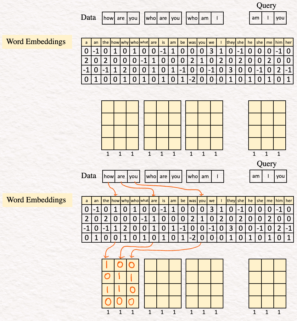
For our example, we have a dataset of three sentences with 3 words (or tokens) for each.

• How are you
• Who are you
• Who am I

And our query is the sentence ‘am I you’.

In real life, a database may contain billions of sentences (think Wikipedia, news archives, journal papers, or any collection of documents) with tens of thousands of max number of tokens. Now that the stage is set, let the process begin :

[1] Embedding : The first step is generating vector embeddings for all the text that we want to be using. To do so, we search for our corresponding words in a table of 22 vectors, where 22 is the vocabulary size for our example.

In real life, the vocabulary size can be tens of thousands. The word embedding dimensions are in the thousands (e.g., 1024, 4096).

By searching for the words how are you in the vocabulary, the word embedding for it looks as this:

[2] Encoding : The next step is encoding the word embedding to obtain a sequence of feature vectors, one per word. For our example, the encoder is a simple perceptron consisting of a Linear layer with a ReLU activation function.

A quick recap:

Linear transformation : The input embedding vector is multiplied by the weight matrix W and then added with the bias vector b,

z = Wx+b, where W is the weight matrix, x is our word embedding and b is the bias vector.

ReLU activation function : Next, we apply the ReLU to this intermediate z.

ReLU returns the element-wise maximum of the input and zero. Mathematically, h = max{0,z}.

Thus, for this example the text embedding looks like this:

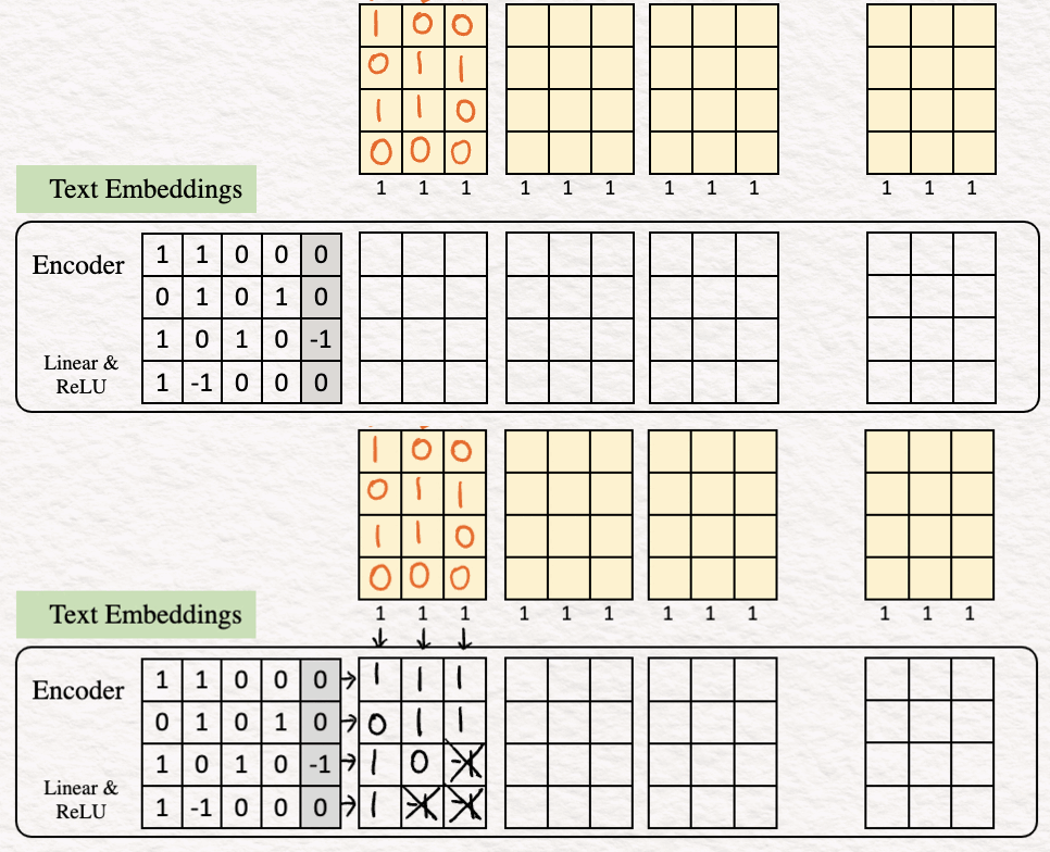
To show how it works, let’s calculate the values for the last column as an example.

Linear transformation :

[1.0 + 1.1 + 0.0 +0.0] + 0 = 1

[0.0 + 1.1 + 0.0 + 1.0] + 0 = 1

[1.0 + (0).1+ 1.0 + 0.0] + (-1) = -1

[1.0 + (-1).1+ 0.0 + 0.0] + 0 = -1

ReLU

max {0,1} =1

max {0,1} = 1

max {0,-1} = 0

max {0,-1} = 0

And thus we get the last column of our feature vector. We can repeat the same steps for the other columns.

[3] Mean Pooling : In this step, we club the feature vectors by averaging over the columns to obtain a single vector. This is often called text embedding or sentence embedding.

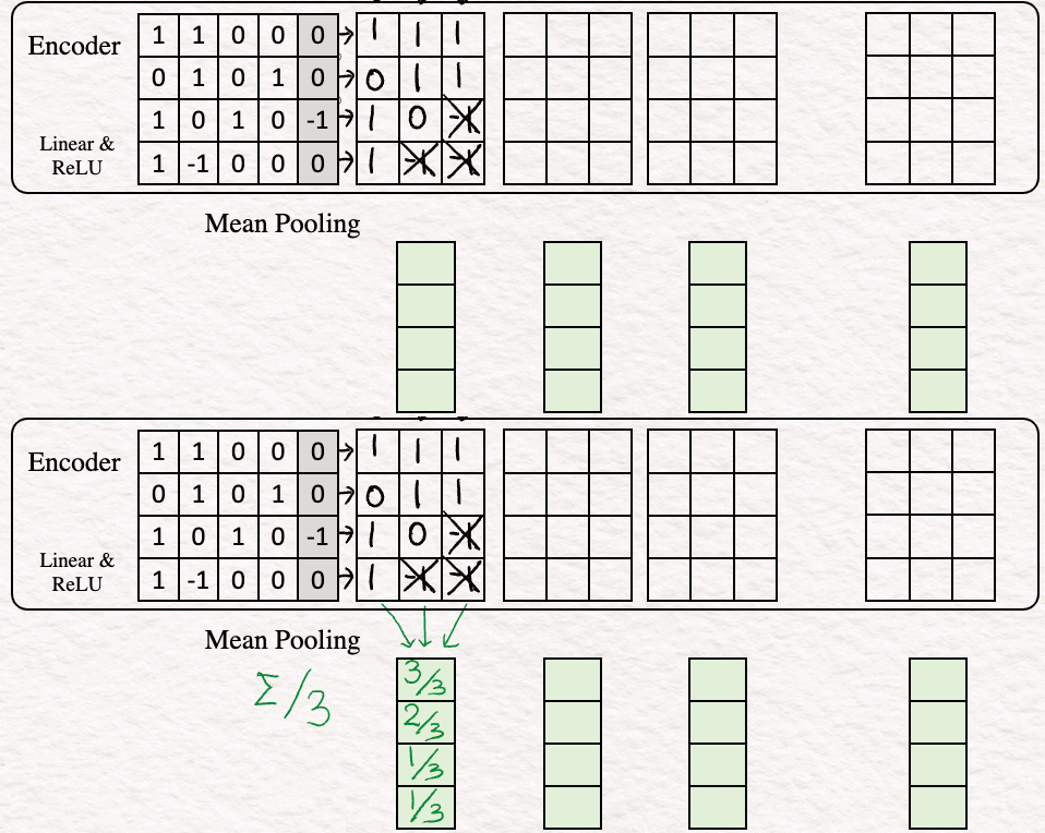
Other techniques for pooling such as CLS, SEP can be used but Mean Pooling is the one used most widely.

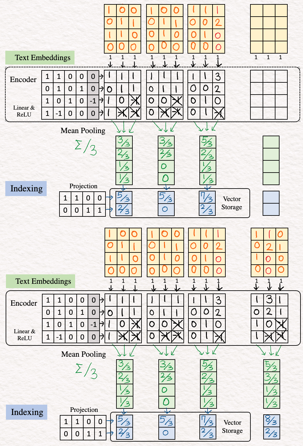
[4] Indexing : The next step involves reducing the dimensions of the text embedding vector, which is done with the help of a projection matrix. This projection matrix could be random. The idea here is to obtain a short representation which would allow faster comparison and retrieval.

This result is kept away in the vector storage.

[5] Repeat : The above steps [1]-[4] are repeated for the other sentences in the dataset “who are you” and “who am I”.

Now that we have indexed our dataset in the vector database, we move on to the actual query and see how these indices play out to give us the solution.

Query : “am I you”

[6] To get started, we repeat the same steps as above — embedding, encoding and indexing to obtain a 2d-vector representation of our query.

[7] Dot Product (Finding Similarity)

Once the previous steps are done, we perform dot products. This is important as these dot products power the idea of comparison between the query vector and our database vectors. To perform this step, we transpose our query vector and multiply it with the database vectors.

[8] Nearest Neighbor

The final step is performing a linear scan to find the largest dot product, which for our example is 60/9. This is the vector representation for “who am I”. In real life, a linear scan could be incredibly slow as it may involve billions of values, the alternative is to use an Approximate Nearest Neighbor (ANN) algorithm like the Hierarchical Navigable Small Worlds (HNSW).

And that brings us to the end of this elegant method.

Thus, by using the vector embeddings of the datasets in the vector database, and performing the steps above, we were able to find the sentence closest to our query. Embedding, encoding, mean pooling, indexing and then dot products form the core of this process.

The ‘large’ picture

However, to bring in the ‘large’ perspective one more time –

• A dataset may contain millions or billions of sentences.
• The number of tokens for each of them can be tens of thousands.
• The word embedding dimensions can be in the thousands.

As we put all of these data and steps together, we are talking about performing operations on dimensions that are mammoth-like in size. And so, to power through this magnificent scale, vector databases come to the rescue. Since we started this article talking about LLMs, it would be a good place to say that because of the scale-handling capability of vector databases, they have come to play a significant role in Retrieval Augmented Generation (RAG). The scalability and speed offered by vector databases enable efficient retrieval for the RAG models, thus paving the way for an efficient generative model.

All in all it is quite right to say that vector databases are powerful. No wonder they have been here for a while — starting their journey of helping recommendation systems to now powering the LLMs, their rule continues. And with the pace vector embeddings are growing for different AI modalities, it seems like vector databases are going to continue their rule for a good amount of time in the future!

P.S. If you would like to work through this exercise on your own, here is a link to a blank template for your use.

Blank Template for hand-exercise

Now go have fun and create some ‘luminous vectoresque’ magic!

Deep Dive into Vector Databases by Hand ✍︎ was originally published in Towards Data Science on Medium, where people are continuing the conversation by highlighting and responding to this story.

Explore what exactly happens behind-the-scenes in Vector Databases

The other day I asked my favorite Large Language Model (LLM) to help me explain vectors to my almost 4-year old. In seconds, it spit out a story filled with mythical creatures and magic and vectors. And Voila! I had a sketch for a new children’s book, and it was impressive because the unicorn was called ‘LuminaVec’.

So, how did the model help weave this creative magic? Well, the answer is by using vectors (in real life) and most probably vector databases. How so? Let me explain.

Vectors and Embedding

First, the model doesn’t understand the exact words I typed in. What helps it understand the words are their numerical representations which are in the form of vectors. These vectors help the model find similarity among the different words while focusing on meaningful information about each. It does this by using embeddings which are low-dimensional vectors that try to capture the semantics and context of the information.

In other words, vectors in an embedding are lists of numbers that specify the position of an object with respect to a reference space. These objects can be features that define a variable in a dataset. With the help of these numerical vector values, we can determine how close or how far one feature is from the other — are they similar (close) or not similar (far)?

Now these vectors are quite powerful but when we are talking about LLMs, we need to be extra cautious about them because of the word ‘large’. As it happens to be with these ‘large’ models, these vectors may quickly become long and more complex, spanning over hundreds or even thousands of dimensions. If not dealt with carefully, the processing speed and mounting expense could become cumbersome very fast!

Vector Databases

To address this issue, we have our mighty warrior : Vector databases.

Vector databases are special databases that contain these vector embeddings. Similar objects have vectors that are closer to each other in the vector database, while dissimilar objects have vectors that are farther apart. So, rather than parsing the data every time a query comes in and generating these vector embeddings, which induces huge resources, it is much faster to run the data through the model once, store it in the vector database and retrieve it as needed. This makes vector databases one of the most powerful solutions addressing the problem of scale and speed for these LLMs.

So, going back to the story about the rainbow unicorn, sparkling magic and powerful vectors — when I had asked the model that question, it may have followed a process as this –

1. The embedding model first transformed the question to a vector embedding.
2. This vector embedding was then compared to the embeddings in the vector database(s) related to fun stories for 5-year olds and vectors.
3. Based on this search and comparison, the vectors that were the most similar were returned. The result should have consisted of a list of vectors ranked in their order of similarity to the query vector.

How does it really work?

To distill things even further, how about we go on a ride to resolve these steps on the micro-level? Time to go back to the basics! Thanks to Prof. Tom Yeh, we have this beautiful handiwork that explains the behind-the-scenes workings of the vectors and vector databases. (All the images below, unless otherwise noted, are by Prof. Tom Yeh from the above-mentioned LinkedIn post, which I have edited with his permission. )

So, here we go:

For our example, we have a dataset of three sentences with 3 words (or tokens) for each.

• How are you
• Who are you
• Who am I

And our query is the sentence ‘am I you’.

In real life, a database may contain billions of sentences (think Wikipedia, news archives, journal papers, or any collection of documents) with tens of thousands of max number of tokens. Now that the stage is set, let the process begin :

[1] Embedding : The first step is generating vector embeddings for all the text that we want to be using. To do so, we search for our corresponding words in a table of 22 vectors, where 22 is the vocabulary size for our example.

In real life, the vocabulary size can be tens of thousands. The word embedding dimensions are in the thousands (e.g., 1024, 4096).

By searching for the words how are you in the vocabulary, the word embedding for it looks as this:

[2] Encoding : The next step is encoding the word embedding to obtain a sequence of feature vectors, one per word. For our example, the encoder is a simple perceptron consisting of a Linear layer with a ReLU activation function.

A quick recap:

Linear transformation : The input embedding vector is multiplied by the weight matrix W and then added with the bias vector b,

z = Wx+b, where W is the weight matrix, x is our word embedding and b is the bias vector.

ReLU activation function : Next, we apply the ReLU to this intermediate z.

ReLU returns the element-wise maximum of the input and zero. Mathematically, h = max{0,z}.

Thus, for this example the text embedding looks like this:

To show how it works, let’s calculate the values for the last column as an example.

Linear transformation :

[1.0 + 1.1 + 0.0 +0.0] + 0 = 1

[0.0 + 1.1 + 0.0 + 1.0] + 0 = 1

[1.0 + (0).1+ 1.0 + 0.0] + (-1) = -1

[1.0 + (-1).1+ 0.0 + 0.0] + 0 = -1

ReLU

max {0,1} =1

max {0,1} = 1

max {0,-1} = 0

max {0,-1} = 0

And thus we get the last column of our feature vector. We can repeat the same steps for the other columns.

[3] Mean Pooling : In this step, we club the feature vectors by averaging over the columns to obtain a single vector. This is often called text embedding or sentence embedding.

Other techniques for pooling such as CLS, SEP can be used but Mean Pooling is the one used most widely.

[4] Indexing : The next step involves reducing the dimensions of the text embedding vector, which is done with the help of a projection matrix. This projection matrix could be random. The idea here is to obtain a short representation which would allow faster comparison and retrieval.

This result is kept away in the vector storage.

[5] Repeat : The above steps [1]-[4] are repeated for the other sentences in the dataset “who are you” and “who am I”.

Now that we have indexed our dataset in the vector database, we move on to the actual query and see how these indices play out to give us the solution.

Query : “am I you”

[6] To get started, we repeat the same steps as above — embedding, encoding and indexing to obtain a 2d-vector representation of our query.

[7] Dot Product (Finding Similarity)

Once the previous steps are done, we perform dot products. This is important as these dot products power the idea of comparison between the query vector and our database vectors. To perform this step, we transpose our query vector and multiply it with the database vectors.

[8] Nearest Neighbor

The final step is performing a linear scan to find the largest dot product, which for our example is 60/9. This is the vector representation for “who am I”. In real life, a linear scan could be incredibly slow as it may involve billions of values, the alternative is to use an Approximate Nearest Neighbor (ANN) algorithm like the Hierarchical Navigable Small Worlds (HNSW).

And that brings us to the end of this elegant method.

Thus, by using the vector embeddings of the datasets in the vector database, and performing the steps above, we were able to find the sentence closest to our query. Embedding, encoding, mean pooling, indexing and then dot products form the core of this process.

The ‘large’ picture

However, to bring in the ‘large’ perspective one more time –

• A dataset may contain millions or billions of sentences.
• The number of tokens for each of them can be tens of thousands.
• The word embedding dimensions can be in the thousands.

As we put all of these data and steps together, we are talking about performing operations on dimensions that are mammoth-like in size. And so, to power through this magnificent scale, vector databases come to the rescue. Since we started this article talking about LLMs, it would be a good place to say that because of the scale-handling capability of vector databases, they have come to play a significant role in Retrieval Augmented Generation (RAG). The scalability and speed offered by vector databases enable efficient retrieval for the RAG models, thus paving the way for an efficient generative model.

All in all it is quite right to say that vector databases are powerful. No wonder they have been here for a while — starting their journey of helping recommendation systems to now powering the LLMs, their rule continues. And with the pace vector embeddings are growing for different AI modalities, it seems like vector databases are going to continue their rule for a good amount of time in the future!

P.S. If you would like to work through this exercise on your own, here is a link to a blank template for your use.

Blank Template for hand-exercise

Now go have fun and create some ‘luminous vectoresque’ magic!

Deep Dive into Vector Databases by Hand ✍︎ was originally published in Towards Data Science on Medium, where people are continuing the conversation by highlighting and responding to this story.

FOLLOW US ON GOOGLE NEWS

Read original article here