
Demystifying Confidence Intervals with Examples
Navigating through uncertainty in data for extracting global statistical insights
Introduction
Confidence intervals are of the most important concepts in statistics. In data science, we often need to calculate statistics for a given data variable. The common problem we encounter is the lack of full data distribution. As a result, statistics are calculated only for a subset of data. The obvious drawback is that the computed statistics of the data subset might differ a lot from the real value, based on all possible values.
It is impossible to completely eliminate this problem, as we will always have some deviation from the real value. Nevertheless, the introduction of confidence intervals with a combination of several algorithms makes it possible to estimate a range of values to which the desired statistic belongs at a certain level of confidence.
Definition
Having understood the ultimate motivation behind confidence intervals, let us understand their definition.
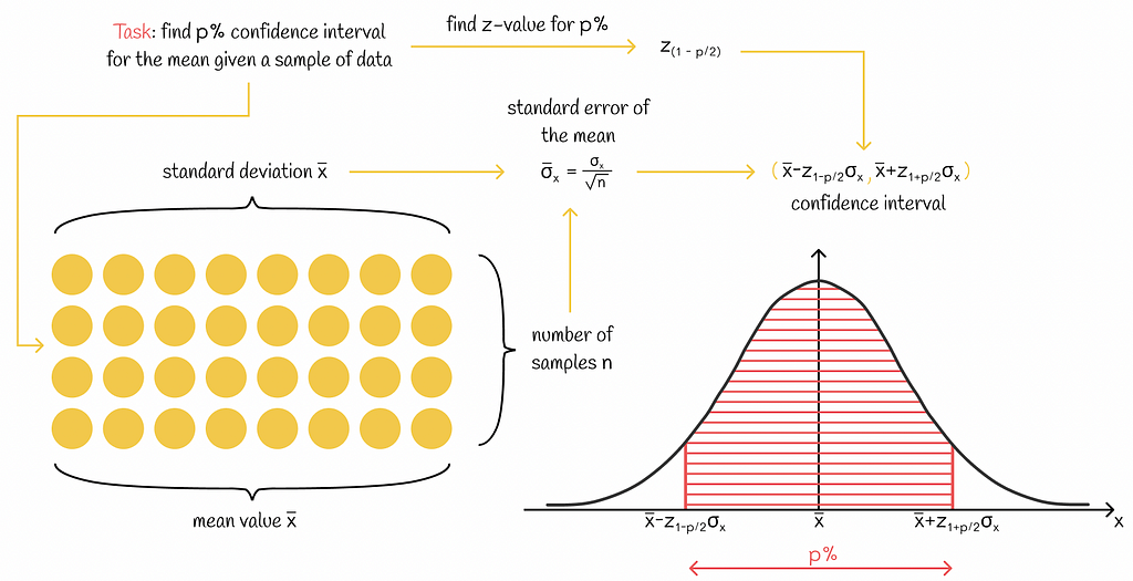
For a given numeric variable and statistic function, the p% confidence interval is a value range that, with the probability of p%, contains the true statistic’s value of that variable.
It is not obligatory, but most of the time, in practice, the confidence level p is chosen as 90%, 95%, or 99%.
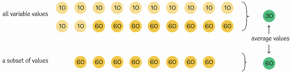
To make things clear, let us consider a simple example. Imagine we want to compute the mean age for a given subset of people so that the final result would be representative for all other people in our set. We do not have information about all people, so to estimate the average age, we will build a confidence interval.
Confidence intervals can be constructed for different statistics. For example, if we wanted to estimate the age median in the group, we would build a confidence interval for the age median.
For now, let us suppose we know how to calculate confidence intervals (the methods will be discussed in the sections below). We will assume that our calculated 95% confidence interval is a range (23, 37). This estimation would exactly mean that, given the data subset above, we can be sure by 95% that the global average of the whole dataset is greater than 23 and less than 37. Only in 5% of cases, the real average value is located outside of this interval.
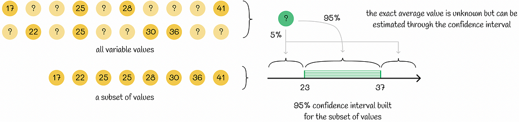
The great thing about confidence intervals is that they usually estimate a given statistic by providing a whole range of values. It allows us to deeper analyse the behaviour of the variable in comparison to a situation where the global value would be represented by only a single value. Furthermore, the confidence level p is usually chosen as high (≥ 90%), meaning that the estimations made by using confidence intervals are almost always correct.
Calculation
As it was noted above, confidence intervals can be estimated for different statistics. Before diving into details, let us first talk about the central limit theorem, which will help us later in constructing confidence intervals.
Confidence intervals for the same variable, statistic, and confidence level can be calculated in several ways and, therefore, be different from each other.
Central limit theorem
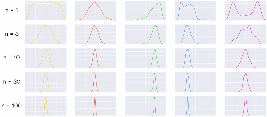
The central limit theorem is a crucial theorem in statistics. Given a random distribution, it states that if we independently sample large random subsets (of size n ≥ 30) from it, calculate the average value in each subset, and plot a distribution of these average values (the mean distribution), then this distribution will be close to normal.
The standard deviation of the mean distribution is called the standard error of the mean (SEM). Similarly, the standard deviation of the median would be called the standard error of the median.
Apart from that, if the standard deviation of the original distribution is known, then the standard error of the mean can be evaluated by the following formula:

Normally, in the numerator of this formula, the standard deviation of all observations should be used. However, in practice, we do not usually have information about all of them but only their subset. Therefore, we use the standard deviation of the sample, assuming that the observations in that sample represent the statistical population well enough.
To put it simply, the standard error of the mean shows how much independent means from sampled distributions vary from each other.
Example
Let us go back to the example of age. Suppose we have a subset of 64 people randomly sampled from the population. The standard deviation of the age in this subset is 18. Since the sample size of 64 is greater than 30, we can calculate the standard error of the age mean for the whole population by using the formula above:

How can this theorem be useful?
At first sight, it seems like this theorem has nothing to do with confidence intervals. Nevertheless, the central limit theorem allows us to precisely calculate confidence intervals for the mean!
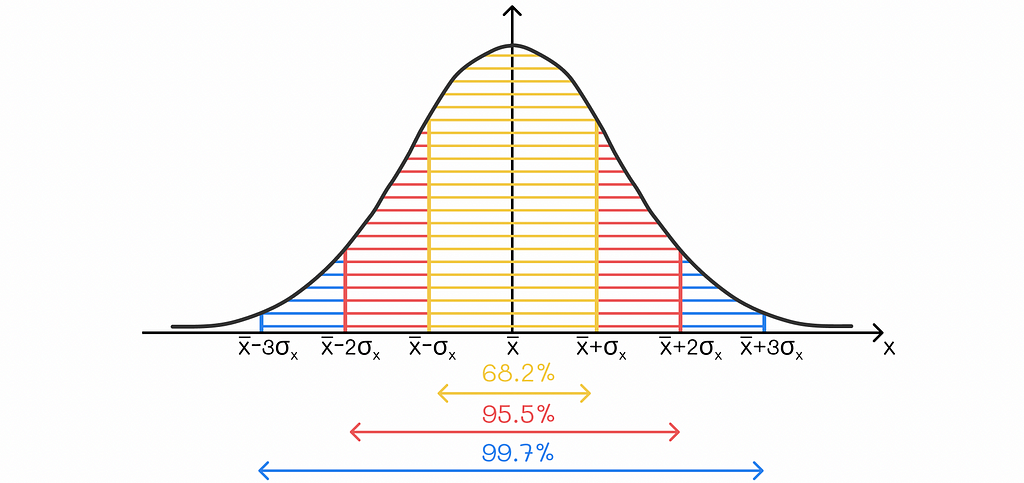
To understand how to do it, let us briefly revise the famous three sigma-rule in statistics. It estimates the percentage of points in a normal distribution that lie at a certain distance from the mean measured by standard deviations. More precisely, the following statements are true:
- 68.2% of the data points lie within z = 1 standard deviation of the mean.
- 95.5% of the data points lie within z = 2 standard deviations of the mean.
- 99.7% of the data points lie within z = 3 standard deviations of the mean.
For other percentages of data points, it is recommended to look for z-values that are already pre-calculated. Each z-value corresponds to the exact number of standard deviations covering a given percentage of data points in a normal distribution.

Let us suppose that we have a data sample from a population, and we would like to find its 95% confidence interval. In the ideal scenario, we would construct the distribution of the mean values to further extract the desired boundaries. Unfortunately, with only the data subset, it would not be possible. At the same time, we do not need to construct the distribution of the mean values since we already know the most important properties about it:
- The distribution of the mean values is normal.
- The standard error of the mean distribution can be calculated.
- Assuming that our subset is a good representation of the whole population, we can claim that the mean value of the given sample is the same as the mean value of the mean distribution. This fact gives us an opportunity to estimate the center of the mean distribution.
This information is perfectly enough to apply the three-sigma rule for the mean distribution! In our case, we would like to calculate a 95% confidence interval; therefore, we should bound the mean distribution by z = 1.96 (value taken from the z-table) standard errors in both directions from the center point.
Example
Let us go back to the example with the age above. We have already calculated the standard error of the mean, which is 2.25.
Let us suppose that we also know the mean age in our sample group, which is equal to 36. Therefore, the mean value of the mean distribution will also be equal to 36. By taking it into consideration, we can compute a confidence interval for the mean. This time, we will use a confidence level of 99%. The equivalent z-value for p = 0.99% is 2.58.
Finally, we should estimate the borders of the interval by knowing that it is located around the center of 36 within z = 2.58 standard errors of the means.
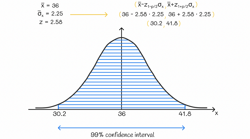
The 99% confidence interval for the example is (30.2, 41.8). The computed result can be interpreted as follows: given information about the age of people in the data subset, there is a 99% probability that the average age of the whole population is greater than 30.2 and less than 41.8.
We could have also built confidence intervals for other confidence levels as well. The chosen confidence level usually depends on the nature of the task. In fact, there is a trade-off between confidence level and precision:
The smaller the confidence level p is, the smaller the corresponding confidence interval is, thus, the statistic’s estimation is more precise.
Other statistics
By robustly combining the central limit theorem with the sigma rule, we have understood how to compute confidence intervals for the mean. However, what would we do if we needed to construct confidence intervals for other statistics like median, interquartile range, standard deviation, etc.? It turns out that is not that easy to do as for the mean, where we can just use the obtained formula.
Nevertheless, there exist algorithms that can provide an approximate result for other statistics. In this section below, we will dive into the most popular one, which is called bootstrap.
Bootstrap
Bootstrap is a methodology used for generating new datasets based on resampling with replacement. The generated dataset is referred to as bootstrapped dataset. In the definition, the replacement indicates that the same sample can be used more than once for the bootstrapped dataset.
The size of the bootstrapped dataset must be the same as the size of the original dataset.
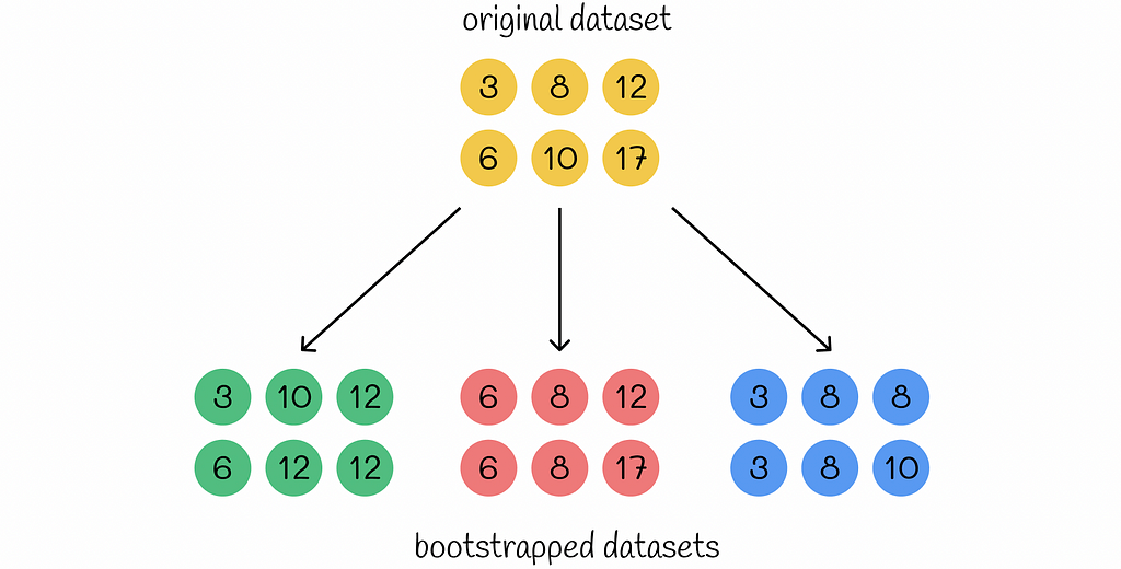
The idea of the bootstrapping is to generate many different versions of the original dataset. If the original dataset is a good representation of the whole population, then the bootstrap method can achieve the effect (even though it is not real) that the bootstrapped datasets are generated from the original population. Because of the replacement strategy, bootstrapped datasets can vary a lot from each other. Therefore, it is especially useful when the original dataset does not contain too many examples that can be precisely analysed. At the same time, bootstrapped datasets can be analysed together to estimate various statistics.
Bootstrap is also used in some machine learning algorithms, like Random Forest or Gradient Boosting, to reduce the chances of overfitting.
Using bootstrap for confidence intervals
Contrary to the previous algorithm, bootsrap fully constructs the distribution of the target statistic. For each generated bootstrapped dataset, the target statistic is calculated and then used as a data point. Ultimately, all the calculated data points form a statistical distribution.
Based on the confidence level p, the bounds covering p% of the data points around the center form a confidence interval.
Code
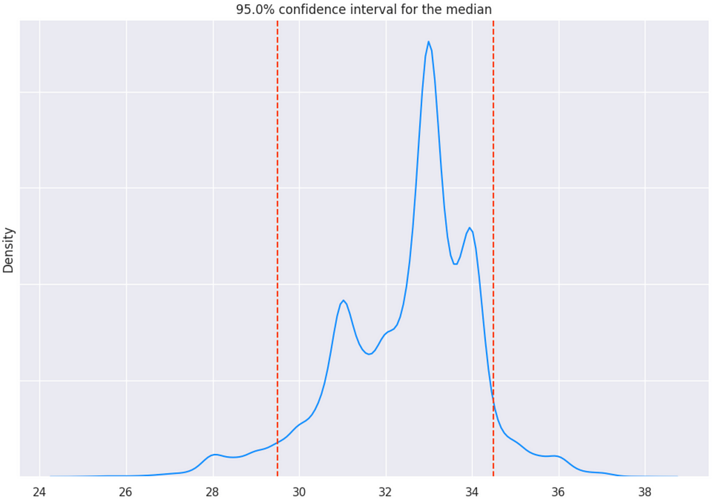
It would be easier to understand the algorithm, by going through the code implementing the bootstrap concept. Let us imagine that we would like to build a 95% confidence interval for the median given 40 sample age observations.
data = [
    33, 37, 21, 27, 34, 33, 36, 46, 40, 25,
    40, 30, 38, 37, 38, 23, 19, 35, 31, 22,
    18, 24, 37, 33, 42, 25, 28, 38, 34, 43,
    20, 26, 32, 29, 31, 41, 23, 28, 36, 34
]
p = 0.95
function = np.median
function_name = 'median'
To achieve that, we will generate n = 1000 bootstrapped datasets of size 30 (the same size as the number of given observations). The larger number of bootstrapped datasets provides more precise estimations.
n = 10000
size = len(data)
datasets = [np.random.choice(data, size, replace=True) for _ in range(n)]
For each bootstrapped dataset, we will calculate its statistic (the median in our case).
statistics = [function(dataset) for dataset in datasets]
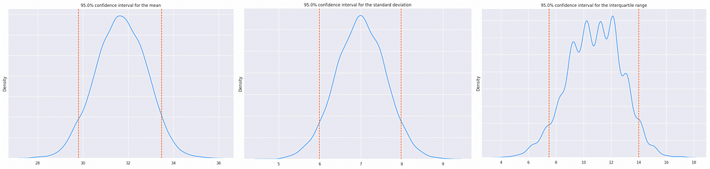
Having calculated all n = 10000 statistics, let us plot their distribution. The 95% confidence interval for the median is located between the 5-th and 95-th quantiles.
lower_quantile = np.quantile(statistics, 1 - p)
upper_quantile = np.quantile(statistics, p)

print(
  f'{p * 100}% confidence interval for the {function_name}:
  ({lower_quantile:.3f}, {upper_quantile:.3f})'
)
plt.figure(figsize=(12, 8))
ax = sns.distplot(statistics, rug=False, hist=False, color='dodgerblue')
ax.yaxis.set_tick_params(labelleft=False)
plt.axvline(lower_quantile, color='orangered', linestyle='--')
plt.axvline(upper_quantile, color='orangered', linestyle='--')
plt.title(f'{p * 100}% confidence interval for the {function_name}')
The analogous strategy can be applied to the computation of other statistics as well.
The significant advantage of using the bootstrap strategy over other methods for confidence interval calculation is that it does not require any assumptions about the initial data. The single requirement for the bootstrap is that the estimated statistic must always have a finite value.
The code used throughout this article can be found here.
Resources
Conclusion
A lack of information is a common issue in Data Science during data analysis. Confidence interval is a powerful tool that probabilistically defines a range of values for global statistics. Combined with the bootstrap methodology or other algorithms, they can produce precise estimations for a large majority of tasks.
All images unless otherwise noted are by the author.
Demystifying Confidence Intervals with Examples was originally published in Towards Data Science on Medium, where people are continuing the conversation by highlighting and responding to this story.
Navigating through uncertainty in data for extracting global statistical insights
Introduction
Confidence intervals are of the most important concepts in statistics. In data science, we often need to calculate statistics for a given data variable. The common problem we encounter is the lack of full data distribution. As a result, statistics are calculated only for a subset of data. The obvious drawback is that the computed statistics of the data subset might differ a lot from the real value, based on all possible values.
It is impossible to completely eliminate this problem, as we will always have some deviation from the real value. Nevertheless, the introduction of confidence intervals with a combination of several algorithms makes it possible to estimate a range of values to which the desired statistic belongs at a certain level of confidence.
Definition
Having understood the ultimate motivation behind confidence intervals, let us understand their definition.
For a given numeric variable and statistic function, the p% confidence interval is a value range that, with the probability of p%, contains the true statistic’s value of that variable.
It is not obligatory, but most of the time, in practice, the confidence level p is chosen as 90%, 95%, or 99%.
To make things clear, let us consider a simple example. Imagine we want to compute the mean age for a given subset of people so that the final result would be representative for all other people in our set. We do not have information about all people, so to estimate the average age, we will build a confidence interval.
Confidence intervals can be constructed for different statistics. For example, if we wanted to estimate the age median in the group, we would build a confidence interval for the age median.
For now, let us suppose we know how to calculate confidence intervals (the methods will be discussed in the sections below). We will assume that our calculated 95% confidence interval is a range (23, 37). This estimation would exactly mean that, given the data subset above, we can be sure by 95% that the global average of the whole dataset is greater than 23 and less than 37. Only in 5% of cases, the real average value is located outside of this interval.
The great thing about confidence intervals is that they usually estimate a given statistic by providing a whole range of values. It allows us to deeper analyse the behaviour of the variable in comparison to a situation where the global value would be represented by only a single value. Furthermore, the confidence level p is usually chosen as high (≥ 90%), meaning that the estimations made by using confidence intervals are almost always correct.
Calculation
As it was noted above, confidence intervals can be estimated for different statistics. Before diving into details, let us first talk about the central limit theorem, which will help us later in constructing confidence intervals.
Confidence intervals for the same variable, statistic, and confidence level can be calculated in several ways and, therefore, be different from each other.
Central limit theorem
The central limit theorem is a crucial theorem in statistics. Given a random distribution, it states that if we independently sample large random subsets (of size n ≥ 30) from it, calculate the average value in each subset, and plot a distribution of these average values (the mean distribution), then this distribution will be close to normal.
The standard deviation of the mean distribution is called the standard error of the mean (SEM). Similarly, the standard deviation of the median would be called the standard error of the median.
Apart from that, if the standard deviation of the original distribution is known, then the standard error of the mean can be evaluated by the following formula:
Normally, in the numerator of this formula, the standard deviation of all observations should be used. However, in practice, we do not usually have information about all of them but only their subset. Therefore, we use the standard deviation of the sample, assuming that the observations in that sample represent the statistical population well enough.
To put it simply, the standard error of the mean shows how much independent means from sampled distributions vary from each other.
Example
Let us go back to the example of age. Suppose we have a subset of 64 people randomly sampled from the population. The standard deviation of the age in this subset is 18. Since the sample size of 64 is greater than 30, we can calculate the standard error of the age mean for the whole population by using the formula above:
How can this theorem be useful?
At first sight, it seems like this theorem has nothing to do with confidence intervals. Nevertheless, the central limit theorem allows us to precisely calculate confidence intervals for the mean!
To understand how to do it, let us briefly revise the famous three sigma-rule in statistics. It estimates the percentage of points in a normal distribution that lie at a certain distance from the mean measured by standard deviations. More precisely, the following statements are true:
- 68.2% of the data points lie within z = 1 standard deviation of the mean.
- 95.5% of the data points lie within z = 2 standard deviations of the mean.
- 99.7% of the data points lie within z = 3 standard deviations of the mean.
For other percentages of data points, it is recommended to look for z-values that are already pre-calculated. Each z-value corresponds to the exact number of standard deviations covering a given percentage of data points in a normal distribution.
Let us suppose that we have a data sample from a population, and we would like to find its 95% confidence interval. In the ideal scenario, we would construct the distribution of the mean values to further extract the desired boundaries. Unfortunately, with only the data subset, it would not be possible. At the same time, we do not need to construct the distribution of the mean values since we already know the most important properties about it:
- The distribution of the mean values is normal.
- The standard error of the mean distribution can be calculated.
- Assuming that our subset is a good representation of the whole population, we can claim that the mean value of the given sample is the same as the mean value of the mean distribution. This fact gives us an opportunity to estimate the center of the mean distribution.
This information is perfectly enough to apply the three-sigma rule for the mean distribution! In our case, we would like to calculate a 95% confidence interval; therefore, we should bound the mean distribution by z = 1.96 (value taken from the z-table) standard errors in both directions from the center point.
Example
Let us go back to the example with the age above. We have already calculated the standard error of the mean, which is 2.25.
Let us suppose that we also know the mean age in our sample group, which is equal to 36. Therefore, the mean value of the mean distribution will also be equal to 36. By taking it into consideration, we can compute a confidence interval for the mean. This time, we will use a confidence level of 99%. The equivalent z-value for p = 0.99% is 2.58.
Finally, we should estimate the borders of the interval by knowing that it is located around the center of 36 within z = 2.58 standard errors of the means.
The 99% confidence interval for the example is (30.2, 41.8). The computed result can be interpreted as follows: given information about the age of people in the data subset, there is a 99% probability that the average age of the whole population is greater than 30.2 and less than 41.8.
We could have also built confidence intervals for other confidence levels as well. The chosen confidence level usually depends on the nature of the task. In fact, there is a trade-off between confidence level and precision:
The smaller the confidence level p is, the smaller the corresponding confidence interval is, thus, the statistic’s estimation is more precise.
Other statistics
By robustly combining the central limit theorem with the sigma rule, we have understood how to compute confidence intervals for the mean. However, what would we do if we needed to construct confidence intervals for other statistics like median, interquartile range, standard deviation, etc.? It turns out that is not that easy to do as for the mean, where we can just use the obtained formula.
Nevertheless, there exist algorithms that can provide an approximate result for other statistics. In this section below, we will dive into the most popular one, which is called bootstrap.
Bootstrap
Bootstrap is a methodology used for generating new datasets based on resampling with replacement. The generated dataset is referred to as bootstrapped dataset. In the definition, the replacement indicates that the same sample can be used more than once for the bootstrapped dataset.
The size of the bootstrapped dataset must be the same as the size of the original dataset.
The idea of the bootstrapping is to generate many different versions of the original dataset. If the original dataset is a good representation of the whole population, then the bootstrap method can achieve the effect (even though it is not real) that the bootstrapped datasets are generated from the original population. Because of the replacement strategy, bootstrapped datasets can vary a lot from each other. Therefore, it is especially useful when the original dataset does not contain too many examples that can be precisely analysed. At the same time, bootstrapped datasets can be analysed together to estimate various statistics.
Bootstrap is also used in some machine learning algorithms, like Random Forest or Gradient Boosting, to reduce the chances of overfitting.
Using bootstrap for confidence intervals
Contrary to the previous algorithm, bootsrap fully constructs the distribution of the target statistic. For each generated bootstrapped dataset, the target statistic is calculated and then used as a data point. Ultimately, all the calculated data points form a statistical distribution.
Based on the confidence level p, the bounds covering p% of the data points around the center form a confidence interval.
Code
It would be easier to understand the algorithm, by going through the code implementing the bootstrap concept. Let us imagine that we would like to build a 95% confidence interval for the median given 40 sample age observations.
data = [
    33, 37, 21, 27, 34, 33, 36, 46, 40, 25,
    40, 30, 38, 37, 38, 23, 19, 35, 31, 22,
    18, 24, 37, 33, 42, 25, 28, 38, 34, 43,
    20, 26, 32, 29, 31, 41, 23, 28, 36, 34
]
p = 0.95
function = np.median
function_name = 'median'
To achieve that, we will generate n = 1000 bootstrapped datasets of size 30 (the same size as the number of given observations). The larger number of bootstrapped datasets provides more precise estimations.
n = 10000
size = len(data)
datasets = [np.random.choice(data, size, replace=True) for _ in range(n)]
For each bootstrapped dataset, we will calculate its statistic (the median in our case).
statistics = [function(dataset) for dataset in datasets]
Having calculated all n = 10000 statistics, let us plot their distribution. The 95% confidence interval for the median is located between the 5-th and 95-th quantiles.
lower_quantile = np.quantile(statistics, 1 - p)
upper_quantile = np.quantile(statistics, p)

print(
  f'{p * 100}% confidence interval for the {function_name}:
  ({lower_quantile:.3f}, {upper_quantile:.3f})'
)
plt.figure(figsize=(12, 8))
ax = sns.distplot(statistics, rug=False, hist=False, color='dodgerblue')
ax.yaxis.set_tick_params(labelleft=False)
plt.axvline(lower_quantile, color='orangered', linestyle='--')
plt.axvline(upper_quantile, color='orangered', linestyle='--')
plt.title(f'{p * 100}% confidence interval for the {function_name}')
The analogous strategy can be applied to the computation of other statistics as well.
The significant advantage of using the bootstrap strategy over other methods for confidence interval calculation is that it does not require any assumptions about the initial data. The single requirement for the bootstrap is that the estimated statistic must always have a finite value.
The code used throughout this article can be found here.
Resources
Conclusion
A lack of information is a common issue in Data Science during data analysis. Confidence interval is a powerful tool that probabilistically defines a range of values for global statistics. Combined with the bootstrap methodology or other algorithms, they can produce precise estimations for a large majority of tasks.
All images unless otherwise noted are by the author.
Demystifying Confidence Intervals with Examples was originally published in Towards Data Science on Medium, where people are continuing the conversation by highlighting and responding to this story.
Denial of responsibility! Techno Blender is an automatic aggregator of the all world’s media. In each content, the hyperlink to the primary source is specified. All trademarks belong to their rightful owners, all materials to their authors. If you are the owner of the content and do not want us to publish your materials, please contact us by email – [email protected]. The content will be deleted within 24 hours.