Dropout in Neural Networks. Dropout layers have been the go-to… | by Harsh Yadav | Jul, 2022

Dropout layers have been the go-to method to reduce the overfitting of neural networks. It is the underworld king of regularisation in the modern era of deep learning.

In this era of deep learning, almost every data scientist must have used the dropout layer at some moment in their career of building neural networks. But, why dropout is so common? How does the dropout layer work internally? What is the problem that it solves? Is there any alternative to dropout?

If you have similar questions regarding dropout layers, then you are in the correct place. In this blog, you will discover the intricacies behind the famous dropout layers. After completing this blog, you would be comfortable answering different queries related to dropout and if you are more of an innovative person, you might come up with a more advanced version of dropout layers.

Let’s start… 🙂

This blog is divided into the following sections:

1. Introduction: The problem it tries to solve
2. What is a dropout?
3. How does it solve the problem?
4. Dropout Implementation
5. Dropout during Inference
6. How it was conceived
7. Tensorflow implementation
8. Conclusion

So before diving deep into its world, let’s address the first question. What is the problem that we are trying to solve?

The deep neural networks have different architectures, sometimes shallow, sometimes very deep trying to generalise on the given dataset. But, in this pursuit of trying too hard to learn different features from the dataset, they sometimes learn the statistical noise in the dataset. This definitely improves the model performance on the training dataset but fails massively on new data points (test dataset). This is the problem of overfitting. To tackle this problem we have various regularisation techniques that penalise the weights of the network but this wasn’t enough.

The best way to reduce overfitting or the best way to regularise a fixed-size model is to get the average predictions from all possible settings of the parameters and aggregate the final output. But, this becomes too computationally expensive and isn’t feasible for a real-time inference/prediction.

The other way is inspired by the ensemble techniques (such as AdaBoost, XGBoost, and Random Forest) where we use multiple neural networks of different architectures. But this requires multiple models to be trained and stored, which over time becomes a huge challenge as the networks grow deeper.

So, we have a great solution known as Dropout Layers.

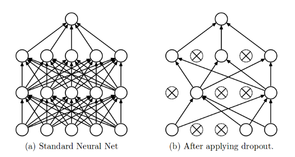
The term “dropout” refers to dropping out the nodes (input and hidden layer) in a neural network (as seen in Figure 1). All the forward and backwards connections with a dropped node are temporarily removed, thus creating a new network architecture out of the parent network. The nodes are dropped by a dropout probability of p.

Let’s try to understand with a given input x: {1, 2, 3, 4, 5} to the fully connected layer. We have a dropout layer with probability p = 0.2 (or keep probability = 0.8). During the forward propagation (training) from the input x, 20% of the nodes would be dropped, i.e. the x could become {1, 0, 3, 4, 5} or {1, 2, 0, 4, 5} and so on. Similarly, it applied to the hidden layers.

For instance, if the hidden layers have 1000 neurons (nodes) and a dropout is applied with drop probability = 0.5, then 500 neurons would be randomly dropped in every iteration (batch).

Generally, for the input layers, the keep probability, i.e. 1- drop probability, is closer to 1, 0.8 being the best as suggested by the authors. For the hidden layers, the greater the drop probability more sparse the model, where 0.5 is the most optimised keep probability, that states dropping 50% of the nodes.

So how does dropout solves the problem of overfitting?

In the overfitting problem, the model learns the statistical noise. To be precise, the main motive of training is to decrease the loss function, given all the units (neurons). So in overfitting, a unit may change in a way that fixes up the mistakes of the other units. This leads to complex co-adaptations, which in turn leads to the overfitting problem because this complex co-adaptation fails to generalise on the unseen dataset.

Now, if we use dropout, it prevents these units to fix up the mistake of other units, thus preventing co-adaptation, as in every iteration the presence of a unit is highly unreliable. So by randomly dropping a few units (nodes), it forces the layers to take more or less responsibility for the input by taking a probabilistic approach.

This ensures that the model is getting generalised and hence reducing the overfitting problem.

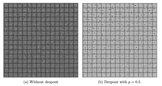
From figure 2, we can easily make out that the hidden layer with dropout is learning more of the generalised features than the co-adaptations in the layer without dropout. It is quite apparent, that dropout breaks such inter-unit relations and focuses more on generalisation.

Enough of the talking! Let’s head to the mathematical explanation of the dropout.

In the original implementation of the dropout layer, during training, a unit (node/neuron) in a layer is selected with a keep probability (1-drop probability). This creates a thinner architecture in the given training batch, and every time this architecture is different.

In the standard neural network, during the forward propagation we have the following equations:

where:
z: denote the vector of output from layer (l + 1) before activation
y: denote the vector of outputs from layer l
w: weight of the layer l
b: bias of the layer l

Further, with the activation function, z is transformed into the output for layer (l+1).

Now, if we have a dropout, the forward propagation equations change in the following way:

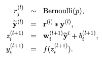
So before we calculate z, the input to the layer is sampled and multiplied element-wise with the independent Bernoulli variables. r denotes the Bernoulli random variables each of which has a probability p of being 1. Basically, r acts as a mask to the input variable, which ensures only a few units are kept according to the keep probability of a dropout. This ensures that we have thinned outputs “y(bar)”, which is given as an input to the layer during feed-forward propagation.

Now, we know the dropout works mathematically but what happens during the inference/prediction? Do we use the network with dropout or do we remove the dropout during inference?

This is one of the most important concepts of dropout which very few data scientists are aware of.

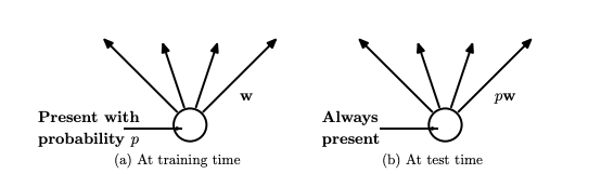
According to the original implementation (Figure 3b) during the inference, we do not use a dropout layer. This means that all the units are considered during the prediction step. But, because of taking all the units/neurons from a layer, the final weights will be larger than expected and to deal with this problem, weights are first scaled by the chosen dropout rate. With this, the network would be able to make accurate predictions.

To be more precise, if a unit is retained with probability p during training, the outgoing weights of that unit are multiplied by p during the prediction stage.

If we follow the original implementation, we need to multiply the weights with the dropout probability during the prediction stage. Just to remove any processing during this stage, we have an implementation known as “inverse dropout”.

The intention of multiplying weights with dropout probability is to ensure that the final weights are of the same scale, thus the predictions are correct. In inverse dropout, this step is performed during the training itself. At the training time, all the weights that remain after the dropout operation is multiplied by the inverse of keep probability, i.e. w * (1/p).

To gain mathematical proof of why both operations are similar on the layer weights, I recommend going through a blog by Lei Mao.

Finally!! We have covered the in-depth analysis of the dropout layers that we use with almost all the neural networks.

Dropouts can be used with most types of neural networks. It is a great tool to reduce overfitting in a model. It is far better than the available regularisation methods and can also be combined with max-norm normalisation which provides a significant boost over just using dropout.

In the upcoming blogs, we would learn more about such basic layers which are used in almost all networks. Batch normalisation, layer normalisation, and attention layers to name a few.

[1] Nitish Srivastava, Dropout: A Simple Way to Prevent Neural Networks from Overfitting, https://jmlr.org/papers/volume15/srivastava14a/srivastava14a.pdf

[2] Jason Brownlee, A Gentle Introduction to Dropout for Regularizing Deep Neural Networks, https://machinelearningmastery.com/dropout-for-regularizing-deep-neural-networks/

[3] Lei Mao, Dropout Explained, https://leimao.github.io/blog/Dropout-Explained/#:~:text=During%20inference%20time%2C%20dropout%20does,were%20multiplied%20by%20pkeep%20.

[4] Juan Miguel, Dropout explained and implementation in Tensorflow, http://laid.delanover.com/dropout-explained-and-implementation-in-tensorflow/

Dropout layers have been the go-to method to reduce the overfitting of neural networks. It is the underworld king of regularisation in the modern era of deep learning.

In this era of deep learning, almost every data scientist must have used the dropout layer at some moment in their career of building neural networks. But, why dropout is so common? How does the dropout layer work internally? What is the problem that it solves? Is there any alternative to dropout?

If you have similar questions regarding dropout layers, then you are in the correct place. In this blog, you will discover the intricacies behind the famous dropout layers. After completing this blog, you would be comfortable answering different queries related to dropout and if you are more of an innovative person, you might come up with a more advanced version of dropout layers.

Let’s start… 🙂

This blog is divided into the following sections:

1. Introduction: The problem it tries to solve
2. What is a dropout?
3. How does it solve the problem?
4. Dropout Implementation
5. Dropout during Inference
6. How it was conceived
7. Tensorflow implementation
8. Conclusion

So before diving deep into its world, let’s address the first question. What is the problem that we are trying to solve?

The deep neural networks have different architectures, sometimes shallow, sometimes very deep trying to generalise on the given dataset. But, in this pursuit of trying too hard to learn different features from the dataset, they sometimes learn the statistical noise in the dataset. This definitely improves the model performance on the training dataset but fails massively on new data points (test dataset). This is the problem of overfitting. To tackle this problem we have various regularisation techniques that penalise the weights of the network but this wasn’t enough.

The best way to reduce overfitting or the best way to regularise a fixed-size model is to get the average predictions from all possible settings of the parameters and aggregate the final output. But, this becomes too computationally expensive and isn’t feasible for a real-time inference/prediction.

The other way is inspired by the ensemble techniques (such as AdaBoost, XGBoost, and Random Forest) where we use multiple neural networks of different architectures. But this requires multiple models to be trained and stored, which over time becomes a huge challenge as the networks grow deeper.

So, we have a great solution known as Dropout Layers.

The term “dropout” refers to dropping out the nodes (input and hidden layer) in a neural network (as seen in Figure 1). All the forward and backwards connections with a dropped node are temporarily removed, thus creating a new network architecture out of the parent network. The nodes are dropped by a dropout probability of p.

Let’s try to understand with a given input x: {1, 2, 3, 4, 5} to the fully connected layer. We have a dropout layer with probability p = 0.2 (or keep probability = 0.8). During the forward propagation (training) from the input x, 20% of the nodes would be dropped, i.e. the x could become {1, 0, 3, 4, 5} or {1, 2, 0, 4, 5} and so on. Similarly, it applied to the hidden layers.

For instance, if the hidden layers have 1000 neurons (nodes) and a dropout is applied with drop probability = 0.5, then 500 neurons would be randomly dropped in every iteration (batch).

Generally, for the input layers, the keep probability, i.e. 1- drop probability, is closer to 1, 0.8 being the best as suggested by the authors. For the hidden layers, the greater the drop probability more sparse the model, where 0.5 is the most optimised keep probability, that states dropping 50% of the nodes.

So how does dropout solves the problem of overfitting?

In the overfitting problem, the model learns the statistical noise. To be precise, the main motive of training is to decrease the loss function, given all the units (neurons). So in overfitting, a unit may change in a way that fixes up the mistakes of the other units. This leads to complex co-adaptations, which in turn leads to the overfitting problem because this complex co-adaptation fails to generalise on the unseen dataset.

Now, if we use dropout, it prevents these units to fix up the mistake of other units, thus preventing co-adaptation, as in every iteration the presence of a unit is highly unreliable. So by randomly dropping a few units (nodes), it forces the layers to take more or less responsibility for the input by taking a probabilistic approach.

This ensures that the model is getting generalised and hence reducing the overfitting problem.

From figure 2, we can easily make out that the hidden layer with dropout is learning more of the generalised features than the co-adaptations in the layer without dropout. It is quite apparent, that dropout breaks such inter-unit relations and focuses more on generalisation.

Enough of the talking! Let’s head to the mathematical explanation of the dropout.

In the original implementation of the dropout layer, during training, a unit (node/neuron) in a layer is selected with a keep probability (1-drop probability). This creates a thinner architecture in the given training batch, and every time this architecture is different.

In the standard neural network, during the forward propagation we have the following equations:

where:
z: denote the vector of output from layer (l + 1) before activation
y: denote the vector of outputs from layer l
w: weight of the layer l
b: bias of the layer l

Further, with the activation function, z is transformed into the output for layer (l+1).

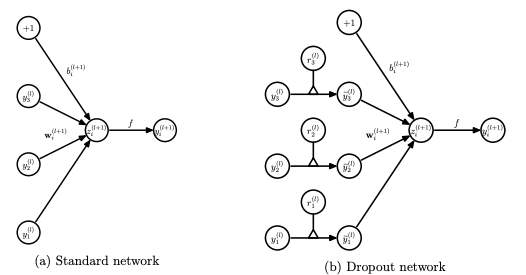
Now, if we have a dropout, the forward propagation equations change in the following way:

So before we calculate z, the input to the layer is sampled and multiplied element-wise with the independent Bernoulli variables. r denotes the Bernoulli random variables each of which has a probability p of being 1. Basically, r acts as a mask to the input variable, which ensures only a few units are kept according to the keep probability of a dropout. This ensures that we have thinned outputs “y(bar)”, which is given as an input to the layer during feed-forward propagation.

Now, we know the dropout works mathematically but what happens during the inference/prediction? Do we use the network with dropout or do we remove the dropout during inference?

This is one of the most important concepts of dropout which very few data scientists are aware of.

According to the original implementation (Figure 3b) during the inference, we do not use a dropout layer. This means that all the units are considered during the prediction step. But, because of taking all the units/neurons from a layer, the final weights will be larger than expected and to deal with this problem, weights are first scaled by the chosen dropout rate. With this, the network would be able to make accurate predictions.

To be more precise, if a unit is retained with probability p during training, the outgoing weights of that unit are multiplied by p during the prediction stage.

If we follow the original implementation, we need to multiply the weights with the dropout probability during the prediction stage. Just to remove any processing during this stage, we have an implementation known as “inverse dropout”.

The intention of multiplying weights with dropout probability is to ensure that the final weights are of the same scale, thus the predictions are correct. In inverse dropout, this step is performed during the training itself. At the training time, all the weights that remain after the dropout operation is multiplied by the inverse of keep probability, i.e. w * (1/p).

To gain mathematical proof of why both operations are similar on the layer weights, I recommend going through a blog by Lei Mao.

Finally!! We have covered the in-depth analysis of the dropout layers that we use with almost all the neural networks.

Dropouts can be used with most types of neural networks. It is a great tool to reduce overfitting in a model. It is far better than the available regularisation methods and can also be combined with max-norm normalisation which provides a significant boost over just using dropout.

In the upcoming blogs, we would learn more about such basic layers which are used in almost all networks. Batch normalisation, layer normalisation, and attention layers to name a few.

[1] Nitish Srivastava, Dropout: A Simple Way to Prevent Neural Networks from Overfitting, https://jmlr.org/papers/volume15/srivastava14a/srivastava14a.pdf

[2] Jason Brownlee, A Gentle Introduction to Dropout for Regularizing Deep Neural Networks, https://machinelearningmastery.com/dropout-for-regularizing-deep-neural-networks/

[3] Lei Mao, Dropout Explained, https://leimao.github.io/blog/Dropout-Explained/#:~:text=During%20inference%20time%2C%20dropout%20does,were%20multiplied%20by%20pkeep%20.

[4] Juan Miguel, Dropout explained and implementation in Tensorflow, http://laid.delanover.com/dropout-explained-and-implementation-in-tensorflow/