
Efficient Object Detection with SSD and YoLO Models — A Comprehensive Beginner’s Guide (Part 3)
Efficient Object Detection with SSD and YoLO Models — A Comprehensive Beginner’s Guide (Part 3)
Learn about single stage object detection models and different trade-offs
In this beginner’s guide series on Object Detection models, we have so far covered the basics of object detection (part-I) and the R-CNN family of object detection models (part-II). We will now focus on some of the famous single-stage object detection models in this article. These models improve upon the speed of inference drastically over multi-stage detectors but fall short of the mAP and other detection metrics. Let’s get into the details for these models.
Single Shot Multi-box Detectors
The Single Shot Multibox Detector (SSD) architecture was presented by Liu et. al. back in 2016 as a highly performant single-stage object detection model. This paper presented a model which was as performant (mAP wise) as Faster R-CNN but faster by a good margin for both training and inference activities.
The main difference between the R-CNN family and SSDs is the missing region proposal component (RPN). The SSD family of models do not start from a selective search algorithm or an RPN to find ROIs. SSD takes a convolutional approach to work on this task of object detection. It produces a predefined number of bounding boxes and corresponding class scores as its final output. It starts off with a large pre-trained network such as VGG-16 which is truncated before any of the classification layers start. This is termed as the base-network in SSD terminology. The base-network is followed by a unique auxiliary structure to produce the required outputs. The following are the key components:
- Multi-Scale Feature Maps: the auxiliary structure after the base-network is a sequence of convolutional layers. These layers progressively decrease the scale or resolution of feature maps. This comes in handy to detect objects of different size (relative to the image). The SSD network takes a convolutional approach to define class scores as well as relative offset values for the bounding boxes. For instance, the network uses a 3x3xp filter on a feature map of m x n x p, where p is the number of channels. The model produces an output for each cell of m x n where the filter is applied.
- Default Anchor Boxes: The network makes use of a set of predefined anchor boxes (at different scales and aspect ratios). For a given feature map of size m x n, k number of such default anchor boxes are applied for each cell. These default anchor boxes are termed as priors in case of SSDs. For each prior in each cell, the model generates c class scores and 4 coordinates for the bounding boxes. Thus, in total for a feature map of size m x n the model generates a total of (c+4)kmn outputs. These outputs are generated from feature maps taken from different depths of the network which is the key to handle multiple sized objects in a single pass.
Figure 1 depicts the high-level architecture for SSD with the base-network as VGG-16 followed by auxiliary convolutional layers to assist with multi-scale feature maps.
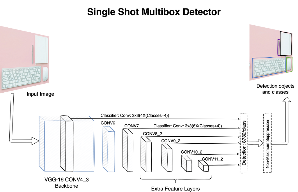
As shown in figure 1, the model generates a total of 8732 predictions which are then analyzed through Non-Maximum Suppression algorithm for finally getting one bounding box per identified object. In the paper, authors present performance metrics (FPS and mAP) for two variants, SSD-300 and SSD-512, where the number denotes the size of input image. Both variants are faster and equally performant (in terms of mAP) as compared to R-CNNs with SSD-300 achieving way more FPS as compared to SSD-512.
As we just discussed, SSD produces a very large number of outputs per feature map. This creates a huge imbalance between positive and negative classes (to ensure coverage, the number of false positives is very large). To handle this and a few other nuances, the authors detail techniques such as hard negative mining and data augmentation. I encourage readers to go through this well drafted paper for more details.
You Look only Once (YOLO)
In the year 2016, another popular single-stage object detection architecture was presented by Redmon et. al. in their paper titled “You Only Look Once: Unified, Real-time Object Detection”. This architecture came up around the same time as SSD but took a slightly different approach to tackle object detection using a single-stage model. Just like the R-CNN family, the YOLO class of models have also evolved over the years with subsequent versions improving upon the previous one. Let us first understand the key aspects of this work.
YOLO is inspired by the GoogleNet architecture for image classification. Similar to GoogleNet, YOLO uses 24 convolutional layers pre-trained on the ImageNet dataset. The pretrained network uses training images of size 224×224 but once trained, the model is used with rescaled inputs of size 448×448. This rescaling was done to ensure that the model picks up small and large objects without issues. It starts off by dividing the input image into an S x S grid (paper mentions a grid of 7×7 for PASCAL VOC dataset). Each cell in the grid predicts B bounding boxes, its objectness score along with confidence score for each of the classes. Thus, similar to SSD each cell in case YOLO outputs 4 coordinates of the bounding boxes plus one objectness score followed by C class prediction probabilities. In total, we get S x S x (Bx5 +C) outputs per input image. The number of output bounding boxes is extremely high, similar to SSDs. These are reduced to a single bounding box per object using NMS algorithm. Figure 2 depicts the overall YOLO setup.
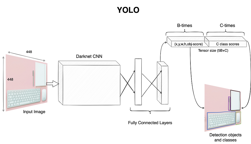
As shown in figure 2, the presence of fully connected layers in YOLO is in contrast with SSD, which is entirely convolutional in design. YOLO is built using an opensource framework called Darknet and boasts of 45FPS inference speed. Its speed comes at the cost of its detection accuracy. Particularly, YOLO has limitations when it comes to identification of smaller objects as well as cases where the objects are overlapping.
YOLOv2 or YOLO-9000 came the very next year (2017) with capability to detect 9000 objects (hence the name) at 45–90 frames per second! One of the minor changes they did was to add an additional step before simply rescaling the inputs to 448×448. Instead, the authors added an additional step where once the original classification model (with input size 224×224) is trained, they rescale the input to 448×448 and fine-tune for a bit more. This enables the model to adapt for larger resolution better and thus improve detection for smaller objects. Also, the convolutional model used is a 30-layer CNN. The second modification was to use anchor boxes and this implementation tries to get the size and number calculated based on the characteristics of the training data (this is in contrast to SSD which simply uses a predefined list of anchor boxes). The final change was to introduce multi-scale training, i.e. instead of just training for a given size the author trained the model at different resolutions to help the model learn features for different sized objects. The changes helped in improving model performance to a good extent (see paper for exact numbers and experiments).
YOLOv3 was presented in 2018 to overcome the mAP shortfall of YOLOv2. This third iteration of the model used a deeper convolutional network with 53 layers as opposed to 24 in the initial version. Another 53 layers are stacked on top of the pre-trained model for detection task. It also uses residual blocks, skip-connections and up-sampling layers to improve performance in general (note that the time the first two version were released some of these concepts were still not commonly used). To better handle different sized objects, this version makes predictions at different depth of the network. The YOLOv3 architecture is depicted in figure 3 for reference.
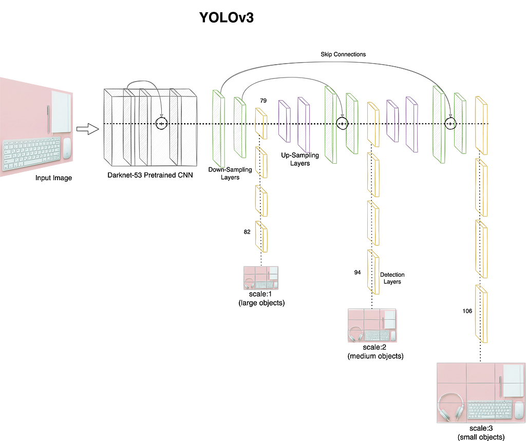
As shown in figure 3, the model branches off from layer 79 and makes predictions at layers 82, 94 and 106 at scales 13×13, 26×26 and 52×52 for large, medium and small sized objects respectively. The model uses 9 anchor boxes, 3 for each scale to handle different shapes as well. This in-turn increases the total number of predictions the model makes per object. The final step is application of NMS to reduce the output to just one bounding box per object detected. Another key change introduced with YOLOv3 was the use of sigmoid loss for class detection in place of softmax. This change helps in handling scenarios where we have overlapping objects.
While the original author of the YOLO model, Joseph Redmon, ceased his work on object detection[1], the overall computer vision community did not stop. There was a subsequent release called YOLOv4 in 2020 followed by another fork titled YOLOv5 a few weeks later (please note that there is no official paper/publication with details of this work). While there are open questions on whether these subsequent releases should carry the YOLO name, it is interesting to see the ideas being refined and carried forward. At the time of writing this article, YOLOv8 is already available for general use while YOLOv9 is pushing efficiencies and other benchmarks even further.
This concludes our brief on different object detection models, both multi-stage and single stage. We have covered key components and major contributions to better understand these models. There are a number of other implementations such as SPP-Net, RetinaNet, etc. which have a different take on the task of object detection. While different, the ideas still conform to the general framework we discussed in this series. In the next article, let us get our hands dirty with some object detection models.
Efficient Object Detection with SSD and YoLO Models — A Comprehensive Beginner’s Guide (Part 3) was originally published in Towards Data Science on Medium, where people are continuing the conversation by highlighting and responding to this story.
Efficient Object Detection with SSD and YoLO Models — A Comprehensive Beginner’s Guide (Part 3)
Learn about single stage object detection models and different trade-offs
In this beginner’s guide series on Object Detection models, we have so far covered the basics of object detection (part-I) and the R-CNN family of object detection models (part-II). We will now focus on some of the famous single-stage object detection models in this article. These models improve upon the speed of inference drastically over multi-stage detectors but fall short of the mAP and other detection metrics. Let’s get into the details for these models.
Single Shot Multi-box Detectors
The Single Shot Multibox Detector (SSD) architecture was presented by Liu et. al. back in 2016 as a highly performant single-stage object detection model. This paper presented a model which was as performant (mAP wise) as Faster R-CNN but faster by a good margin for both training and inference activities.
The main difference between the R-CNN family and SSDs is the missing region proposal component (RPN). The SSD family of models do not start from a selective search algorithm or an RPN to find ROIs. SSD takes a convolutional approach to work on this task of object detection. It produces a predefined number of bounding boxes and corresponding class scores as its final output. It starts off with a large pre-trained network such as VGG-16 which is truncated before any of the classification layers start. This is termed as the base-network in SSD terminology. The base-network is followed by a unique auxiliary structure to produce the required outputs. The following are the key components:
- Multi-Scale Feature Maps: the auxiliary structure after the base-network is a sequence of convolutional layers. These layers progressively decrease the scale or resolution of feature maps. This comes in handy to detect objects of different size (relative to the image). The SSD network takes a convolutional approach to define class scores as well as relative offset values for the bounding boxes. For instance, the network uses a 3x3xp filter on a feature map of m x n x p, where p is the number of channels. The model produces an output for each cell of m x n where the filter is applied.
- Default Anchor Boxes: The network makes use of a set of predefined anchor boxes (at different scales and aspect ratios). For a given feature map of size m x n, k number of such default anchor boxes are applied for each cell. These default anchor boxes are termed as priors in case of SSDs. For each prior in each cell, the model generates c class scores and 4 coordinates for the bounding boxes. Thus, in total for a feature map of size m x n the model generates a total of (c+4)kmn outputs. These outputs are generated from feature maps taken from different depths of the network which is the key to handle multiple sized objects in a single pass.
Figure 1 depicts the high-level architecture for SSD with the base-network as VGG-16 followed by auxiliary convolutional layers to assist with multi-scale feature maps.
As shown in figure 1, the model generates a total of 8732 predictions which are then analyzed through Non-Maximum Suppression algorithm for finally getting one bounding box per identified object. In the paper, authors present performance metrics (FPS and mAP) for two variants, SSD-300 and SSD-512, where the number denotes the size of input image. Both variants are faster and equally performant (in terms of mAP) as compared to R-CNNs with SSD-300 achieving way more FPS as compared to SSD-512.
As we just discussed, SSD produces a very large number of outputs per feature map. This creates a huge imbalance between positive and negative classes (to ensure coverage, the number of false positives is very large). To handle this and a few other nuances, the authors detail techniques such as hard negative mining and data augmentation. I encourage readers to go through this well drafted paper for more details.
You Look only Once (YOLO)
In the year 2016, another popular single-stage object detection architecture was presented by Redmon et. al. in their paper titled “You Only Look Once: Unified, Real-time Object Detection”. This architecture came up around the same time as SSD but took a slightly different approach to tackle object detection using a single-stage model. Just like the R-CNN family, the YOLO class of models have also evolved over the years with subsequent versions improving upon the previous one. Let us first understand the key aspects of this work.
YOLO is inspired by the GoogleNet architecture for image classification. Similar to GoogleNet, YOLO uses 24 convolutional layers pre-trained on the ImageNet dataset. The pretrained network uses training images of size 224×224 but once trained, the model is used with rescaled inputs of size 448×448. This rescaling was done to ensure that the model picks up small and large objects without issues. It starts off by dividing the input image into an S x S grid (paper mentions a grid of 7×7 for PASCAL VOC dataset). Each cell in the grid predicts B bounding boxes, its objectness score along with confidence score for each of the classes. Thus, similar to SSD each cell in case YOLO outputs 4 coordinates of the bounding boxes plus one objectness score followed by C class prediction probabilities. In total, we get S x S x (Bx5 +C) outputs per input image. The number of output bounding boxes is extremely high, similar to SSDs. These are reduced to a single bounding box per object using NMS algorithm. Figure 2 depicts the overall YOLO setup.
As shown in figure 2, the presence of fully connected layers in YOLO is in contrast with SSD, which is entirely convolutional in design. YOLO is built using an opensource framework called Darknet and boasts of 45FPS inference speed. Its speed comes at the cost of its detection accuracy. Particularly, YOLO has limitations when it comes to identification of smaller objects as well as cases where the objects are overlapping.
YOLOv2 or YOLO-9000 came the very next year (2017) with capability to detect 9000 objects (hence the name) at 45–90 frames per second! One of the minor changes they did was to add an additional step before simply rescaling the inputs to 448×448. Instead, the authors added an additional step where once the original classification model (with input size 224×224) is trained, they rescale the input to 448×448 and fine-tune for a bit more. This enables the model to adapt for larger resolution better and thus improve detection for smaller objects. Also, the convolutional model used is a 30-layer CNN. The second modification was to use anchor boxes and this implementation tries to get the size and number calculated based on the characteristics of the training data (this is in contrast to SSD which simply uses a predefined list of anchor boxes). The final change was to introduce multi-scale training, i.e. instead of just training for a given size the author trained the model at different resolutions to help the model learn features for different sized objects. The changes helped in improving model performance to a good extent (see paper for exact numbers and experiments).
YOLOv3 was presented in 2018 to overcome the mAP shortfall of YOLOv2. This third iteration of the model used a deeper convolutional network with 53 layers as opposed to 24 in the initial version. Another 53 layers are stacked on top of the pre-trained model for detection task. It also uses residual blocks, skip-connections and up-sampling layers to improve performance in general (note that the time the first two version were released some of these concepts were still not commonly used). To better handle different sized objects, this version makes predictions at different depth of the network. The YOLOv3 architecture is depicted in figure 3 for reference.
As shown in figure 3, the model branches off from layer 79 and makes predictions at layers 82, 94 and 106 at scales 13×13, 26×26 and 52×52 for large, medium and small sized objects respectively. The model uses 9 anchor boxes, 3 for each scale to handle different shapes as well. This in-turn increases the total number of predictions the model makes per object. The final step is application of NMS to reduce the output to just one bounding box per object detected. Another key change introduced with YOLOv3 was the use of sigmoid loss for class detection in place of softmax. This change helps in handling scenarios where we have overlapping objects.
While the original author of the YOLO model, Joseph Redmon, ceased his work on object detection[1], the overall computer vision community did not stop. There was a subsequent release called YOLOv4 in 2020 followed by another fork titled YOLOv5 a few weeks later (please note that there is no official paper/publication with details of this work). While there are open questions on whether these subsequent releases should carry the YOLO name, it is interesting to see the ideas being refined and carried forward. At the time of writing this article, YOLOv8 is already available for general use while YOLOv9 is pushing efficiencies and other benchmarks even further.
This concludes our brief on different object detection models, both multi-stage and single stage. We have covered key components and major contributions to better understand these models. There are a number of other implementations such as SPP-Net, RetinaNet, etc. which have a different take on the task of object detection. While different, the ideas still conform to the general framework we discussed in this series. In the next article, let us get our hands dirty with some object detection models.
Efficient Object Detection with SSD and YoLO Models — A Comprehensive Beginner’s Guide (Part 3) was originally published in Towards Data Science on Medium, where people are continuing the conversation by highlighting and responding to this story.
Denial of responsibility! Techno Blender is an automatic aggregator of the all world’s media. In each content, the hyperlink to the primary source is specified. All trademarks belong to their rightful owners, all materials to their authors. If you are the owner of the content and do not want us to publish your materials, please contact us by email – [email protected]. The content will be deleted within 24 hours.