
Enhancing Cancer Detection with StyleGAN-2 ADA
Data augmentation for data-deficient deep neural networks.
By: Ian Stebbins, Benjamin Goldfried, Ben Maizes
Intro
Often for many domain-specific problems, a lack of data can hinder the effectiveness and even disallow the use of deep neural networks. Recent architectures of Generative Adversarial Networks (GANs), however, allow us to synthetically augment data, by creating new samples that capture intricate details, textures, and variations in the data distribution. This synthetic data can act as additional training input for deep neural networks, thus making domain tasks with limited data more feasible.
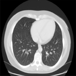
In this project, we applied NVIDIA StyleGAN-2 with Adaptive Discriminator Augmentation (ADA) to a small Chest CT-Scan Dataset (Licensed under Database: Open Database, Contents: © Original Authors)[1]. Additionally, we built a CNN classifier to distinguish normal scans from those with tumors. By injecting varying proportions of synthetically generated data into the training of different models, we were able to evaluate the performance differences between models with all real data and those with a real-synthetic mix.
StyleGAN-2 ADA
StyleGAN-2 with ADA was first introduced by NVIDIA in the NeurIPS 2020 paper: “Training Generative Adversarial Networks with Limited Data” [2]. In the past, training GANs on small datasets typically led to the network discriminator overfitting. Thus rather than learning to distinguish between real and generated data, the discriminator tended to memorize the patterns of noise and outliers of the training set, rather than learn the general trends of the data distribution. To combat this, ADA dynamically adjusts the strength of data augmentation based on the degree of overfitting observed during training. This helps the model to generalize better and leads to better GAN performance on smaller datasets.
Augmenting The Dataset
To use the StyleGAN-2 ADA model, we used the official NVIDIA model implementation from GitHub, which can be found here. Note that this is the StyleGAN-3 repo but StyleGAN-2 can still be run.
!git clone https://github.com/NVlabs/stylegan3
Depending on your setup you may have to install dependencies and do some other preprocessing. For example, we chose to resize and shrink our dataset images to 224×224 since we only had access to a single GPU, and using larger image sizes is much more computationally expensive. We chose to use 224×224 because ResNet, the pre-trained model we chose for the CNN, is optimized to work with this size of image.
!pip install pillow
from PIL import Image
import os

'''Loops through the files in an input folder (input_folder), resizes them to a
specified new size (new_size), an adds them to an output folder (output_folder).'''
def resize_images_in_folder(input_folder, output_folder, new_size):
    # Loop through all files in the input folder
    for filename in os.listdir(input_folder):
        input_path = os.path.join(input_folder, filename)

        # Check if the file is an image
        if os.path.isfile(input_path) and filename.lower().endswith(('.png', '.jpg', '.jpeg', '.gif')):
            # Open the image file
            image = Image.open(input_path)

            #Convert to RGB
            image = image.convert('RGB')

            # Resize the image
            resized_image = image.resize(new_size)

            # Generate the output file path
            output_path = os.path.join(output_folder, filename)

            # Save the resized image to the output folder
            resized_image.save(output_path)

            print(f"Resized {filename} and saved to {output_path}")
To begin the training process, navigate to the directory where you cloned the repo and then run the following.
import os

!python dataset_tool.py --source= "Raw Data Directory" --dest="Output Directory" --resolution='256x256'

# Training
EXPERIMENTS = "Output directory where the Network Pickle File will be saved""
DATA = "Your Training DataSet Directory"
SNAP = 10
KIMG = 80

# Build the command and run it
cmd = f"/usr/bin/python3 /content/stylegan3/train.py --snap {SNAP} --outdir {EXPERIMENTS} --data {DATA}  --kimg {KIMG} --cfg stylegan2 --gpus 1 --batch 8 --gamma 50"
!{cmd}
SNAP refers to the number of Ticks (training steps where information is displayed) after which you would like to take a snapshot of your network and save it to a pickle file.
KIMG refers to the number of thousands of images you want to feed into your GAN.
GAMMA determines how strongly the regularization affects the discriminator.
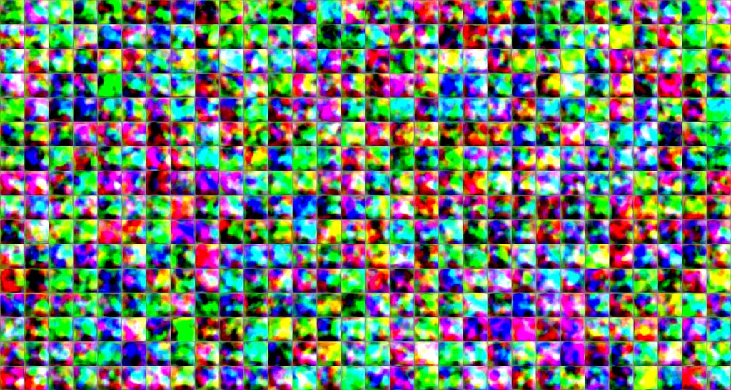
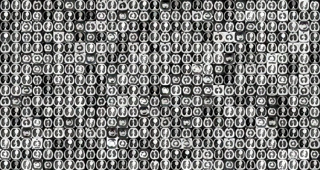
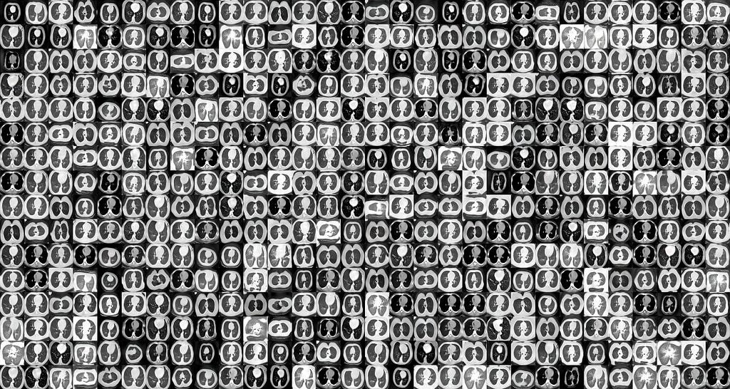
Once your model has finished training (this can take multiple hours depending on your compute resources) you can now use your trained network to generate images.
pickle_file = "Network_Snapshot.pkl"
model_path = f'Path to Pickle File/{pickle_file}'
SAMPLES = Number of samples you want to generate
!python /content/stylegan3/gen_images.py --outdir=Output Directory --trunc=1 --seeds {SAMPLES} \
    --network=$model_path

Transfer Learning & Convolutional Neural Network
To benchmark the effectiveness of our synthetically generated data, we first trained a CNN model on our original data. Once we had a benchmark accuracy on the test set, we re-trained the model with increasing amounts of synthetic data in the training mix.
To feed our data into the model we used Keras data generators which flow the samples directly from a specified directory into the model. The original dataset has 4 classes for different types of cancer, however, for simplicity, we turned this into a binary classification problem. The two classes we decided to work with from the original Kaggle dataset were the normal and squamous classes.
# Define directories for training, validation, and test datasets
train_dir = 'Your training data directory'
test_dir = 'Your testing data directory'
val_dir = 'Your validation data directory'

# Utilize data genarators to flow directly from directories
train_generator = train_datagen.flow_from_directory(
    train_dir,
    target_size=(224, 224),
    batch_size=20,
    class_mode='binary',  #Use 'categorical' for multi-class classification
    shuffle=True,
    seed=42 )

val_generator = val_datagen.flow_from_directory(
    val_dir,
    target_size=(224, 224),
    batch_size=20,
    class_mode='binary',
    shuffle=True )

test_generator = test_datagen.flow_from_directory(
    test_dir,
    target_size=(224, 224),
    batch_size=20,
    class_mode='binary',
    shuffle=True )
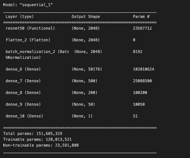
To build our model, we began by using the ResNet50 base architecture and model weights. We chose to use ResNet50 due to its moderate-size architecture, good documentation, and ease of use through Keras. After importing ResNet50 with the Imagenet model weights, we then froze the ResNet50 layers and added trainable dense layers on top to help the network learn our specific classification task.
We also chose to incorporate batch normalization, which can lead to faster convergence and more stable training by normalizing layer inputs and reducing internal covariate shift [3]. Additionally, it can provide a regularization effect that can help prevent overfitting in our added trainable dense layers.
Originally, our model was not performing well. We solved this issue by switching our activation function from ReLU to leaky ReLU. This suggested that our network may have been facing the dying ReLU or dead neuron problem. In short, since the gradient of ReLU will always be zero for negative numbers, this can lead to neurons “dying” and not contributing to the network [4][5]. Since leaky ReLU is nonzero for negative values, using it as an activation function can help combat this issue.
Results
To test our synthetic data, we trained the above CNN on 5 separate instances with 0%, 25%, 50%, 75%, and 100% additional synthetic samples. For example, 0% synthetic samples meant that the data was all original, while 100% meant the training set contained equal amounts of original and synthetic data. For each network, we then evaluated the performance using an accuracy metric on a real set of unseen test data. The plot below visualizes how different proportions of synthetic data affect the testing accuracy.
Training the model was unstable, thus we ruled out iterations where the accuracy was 1.0 or extremely low. This helped us avoid training iterations that were under or over fit.
We can see that from 0 to 25% we see a sharp increase in the testing accuracy, suggesting that even augmenting the dataset by a small amount can have a large impact on problems where the data is initially minimal.
Since we only trained our GAN on 80 KIMG (due to compute limitations) the quality of our synthetic data could have potentially been better, given more GAN training iterations. Notably, an increase in synthetic data quality could also influence the graph above. We hypothesize that an increase in synthetic quality will also lead to an increase in the optimal proportion of synthetic data used in training. Further, if the synthetic images were better able to fit the real distribution of our training data, we could incorporate more of them in model training without overfitting.
Conclusion
In this project, using GANs for the augmentation of limited data has shown to be an effective technique for expanding training sets and more importantly, improving classification accuracy. While we opted for a small and basic problem, this could easily be upscaled in a few ways. Future work may include using more computational resources to get better synthetic samples, introducing more classes into the classification task (making it a multi-class problem), and experimenting with newer GAN architectures. Regardless, using GANs to augment small datasets can now bring many previously data-limited problems into the scope of deep neural networks.
Kaggle Dataset
We compiled our augmented and resized images into the following Kaggle dataset. This contains 501 normal and 501 squamous 224×224 synthetic images which can be used for further experimentation.
Citations
[1] Hany, Mohamed, Chest CT-Scan images Dataset, Kaggle (2020).
[2] Karras, Tero, et al, Training Generative Adversarial Networks with Limited Data (2020), Advances in neural information processing systems 2020.
[3] Ioffe, Sergey, and Christian Szegedy, Batch normalization: Accelerating deep network training by reducing internal covariate shift, (2015), International conference on machine learning. pmlr, 2015.
[4] He, Kaiming, et al, Delving deep into rectifiers: Surpassing human-level performance on imagenet classification, (2015), Proceedings of the IEEE international conference on computer vision. 2015.
[5]Bai, Yuhan, RELU-function and derived function review, (2022), SHS Web of Conferences. Vol. 144. EDP Sciences, 2022.
Enhancing Cancer Detection with StyleGAN-2 ADA was originally published in Towards Data Science on Medium, where people are continuing the conversation by highlighting and responding to this story.
Data augmentation for data-deficient deep neural networks.
By: Ian Stebbins, Benjamin Goldfried, Ben Maizes
Intro
Often for many domain-specific problems, a lack of data can hinder the effectiveness and even disallow the use of deep neural networks. Recent architectures of Generative Adversarial Networks (GANs), however, allow us to synthetically augment data, by creating new samples that capture intricate details, textures, and variations in the data distribution. This synthetic data can act as additional training input for deep neural networks, thus making domain tasks with limited data more feasible.
In this project, we applied NVIDIA StyleGAN-2 with Adaptive Discriminator Augmentation (ADA) to a small Chest CT-Scan Dataset (Licensed under Database: Open Database, Contents: © Original Authors)[1]. Additionally, we built a CNN classifier to distinguish normal scans from those with tumors. By injecting varying proportions of synthetically generated data into the training of different models, we were able to evaluate the performance differences between models with all real data and those with a real-synthetic mix.
StyleGAN-2 ADA
StyleGAN-2 with ADA was first introduced by NVIDIA in the NeurIPS 2020 paper: “Training Generative Adversarial Networks with Limited Data” [2]. In the past, training GANs on small datasets typically led to the network discriminator overfitting. Thus rather than learning to distinguish between real and generated data, the discriminator tended to memorize the patterns of noise and outliers of the training set, rather than learn the general trends of the data distribution. To combat this, ADA dynamically adjusts the strength of data augmentation based on the degree of overfitting observed during training. This helps the model to generalize better and leads to better GAN performance on smaller datasets.
Augmenting The Dataset
To use the StyleGAN-2 ADA model, we used the official NVIDIA model implementation from GitHub, which can be found here. Note that this is the StyleGAN-3 repo but StyleGAN-2 can still be run.
!git clone https://github.com/NVlabs/stylegan3
Depending on your setup you may have to install dependencies and do some other preprocessing. For example, we chose to resize and shrink our dataset images to 224×224 since we only had access to a single GPU, and using larger image sizes is much more computationally expensive. We chose to use 224×224 because ResNet, the pre-trained model we chose for the CNN, is optimized to work with this size of image.
!pip install pillow
from PIL import Image
import os

'''Loops through the files in an input folder (input_folder), resizes them to a
specified new size (new_size), an adds them to an output folder (output_folder).'''
def resize_images_in_folder(input_folder, output_folder, new_size):
    # Loop through all files in the input folder
    for filename in os.listdir(input_folder):
        input_path = os.path.join(input_folder, filename)

        # Check if the file is an image
        if os.path.isfile(input_path) and filename.lower().endswith(('.png', '.jpg', '.jpeg', '.gif')):
            # Open the image file
            image = Image.open(input_path)

            #Convert to RGB
            image = image.convert('RGB')

            # Resize the image
            resized_image = image.resize(new_size)

            # Generate the output file path
            output_path = os.path.join(output_folder, filename)

            # Save the resized image to the output folder
            resized_image.save(output_path)

            print(f"Resized {filename} and saved to {output_path}")
To begin the training process, navigate to the directory where you cloned the repo and then run the following.
import os

!python dataset_tool.py --source= "Raw Data Directory" --dest="Output Directory" --resolution='256x256'

# Training
EXPERIMENTS = "Output directory where the Network Pickle File will be saved""
DATA = "Your Training DataSet Directory"
SNAP = 10
KIMG = 80

# Build the command and run it
cmd = f"/usr/bin/python3 /content/stylegan3/train.py --snap {SNAP} --outdir {EXPERIMENTS} --data {DATA}  --kimg {KIMG} --cfg stylegan2 --gpus 1 --batch 8 --gamma 50"
!{cmd}
SNAP refers to the number of Ticks (training steps where information is displayed) after which you would like to take a snapshot of your network and save it to a pickle file.
KIMG refers to the number of thousands of images you want to feed into your GAN.
GAMMA determines how strongly the regularization affects the discriminator.

Once your model has finished training (this can take multiple hours depending on your compute resources) you can now use your trained network to generate images.
pickle_file = "Network_Snapshot.pkl"
model_path = f'Path to Pickle File/{pickle_file}'
SAMPLES = Number of samples you want to generate
!python /content/stylegan3/gen_images.py --outdir=Output Directory --trunc=1 --seeds {SAMPLES} \
    --network=$model_path
Transfer Learning & Convolutional Neural Network
To benchmark the effectiveness of our synthetically generated data, we first trained a CNN model on our original data. Once we had a benchmark accuracy on the test set, we re-trained the model with increasing amounts of synthetic data in the training mix.
To feed our data into the model we used Keras data generators which flow the samples directly from a specified directory into the model. The original dataset has 4 classes for different types of cancer, however, for simplicity, we turned this into a binary classification problem. The two classes we decided to work with from the original Kaggle dataset were the normal and squamous classes.
# Define directories for training, validation, and test datasets
train_dir = 'Your training data directory'
test_dir = 'Your testing data directory'
val_dir = 'Your validation data directory'

# Utilize data genarators to flow directly from directories
train_generator = train_datagen.flow_from_directory(
    train_dir,
    target_size=(224, 224),
    batch_size=20,
    class_mode='binary',  #Use 'categorical' for multi-class classification
    shuffle=True,
    seed=42 )

val_generator = val_datagen.flow_from_directory(
    val_dir,
    target_size=(224, 224),
    batch_size=20,
    class_mode='binary',
    shuffle=True )

test_generator = test_datagen.flow_from_directory(
    test_dir,
    target_size=(224, 224),
    batch_size=20,
    class_mode='binary',
    shuffle=True )
To build our model, we began by using the ResNet50 base architecture and model weights. We chose to use ResNet50 due to its moderate-size architecture, good documentation, and ease of use through Keras. After importing ResNet50 with the Imagenet model weights, we then froze the ResNet50 layers and added trainable dense layers on top to help the network learn our specific classification task.
We also chose to incorporate batch normalization, which can lead to faster convergence and more stable training by normalizing layer inputs and reducing internal covariate shift [3]. Additionally, it can provide a regularization effect that can help prevent overfitting in our added trainable dense layers.
Originally, our model was not performing well. We solved this issue by switching our activation function from ReLU to leaky ReLU. This suggested that our network may have been facing the dying ReLU or dead neuron problem. In short, since the gradient of ReLU will always be zero for negative numbers, this can lead to neurons “dying” and not contributing to the network [4][5]. Since leaky ReLU is nonzero for negative values, using it as an activation function can help combat this issue.
Results
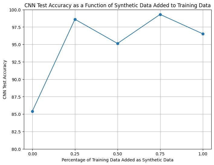
To test our synthetic data, we trained the above CNN on 5 separate instances with 0%, 25%, 50%, 75%, and 100% additional synthetic samples. For example, 0% synthetic samples meant that the data was all original, while 100% meant the training set contained equal amounts of original and synthetic data. For each network, we then evaluated the performance using an accuracy metric on a real set of unseen test data. The plot below visualizes how different proportions of synthetic data affect the testing accuracy.
Training the model was unstable, thus we ruled out iterations where the accuracy was 1.0 or extremely low. This helped us avoid training iterations that were under or over fit.
We can see that from 0 to 25% we see a sharp increase in the testing accuracy, suggesting that even augmenting the dataset by a small amount can have a large impact on problems where the data is initially minimal.
Since we only trained our GAN on 80 KIMG (due to compute limitations) the quality of our synthetic data could have potentially been better, given more GAN training iterations. Notably, an increase in synthetic data quality could also influence the graph above. We hypothesize that an increase in synthetic quality will also lead to an increase in the optimal proportion of synthetic data used in training. Further, if the synthetic images were better able to fit the real distribution of our training data, we could incorporate more of them in model training without overfitting.
Conclusion
In this project, using GANs for the augmentation of limited data has shown to be an effective technique for expanding training sets and more importantly, improving classification accuracy. While we opted for a small and basic problem, this could easily be upscaled in a few ways. Future work may include using more computational resources to get better synthetic samples, introducing more classes into the classification task (making it a multi-class problem), and experimenting with newer GAN architectures. Regardless, using GANs to augment small datasets can now bring many previously data-limited problems into the scope of deep neural networks.
Kaggle Dataset
We compiled our augmented and resized images into the following Kaggle dataset. This contains 501 normal and 501 squamous 224×224 synthetic images which can be used for further experimentation.
Citations
[1] Hany, Mohamed, Chest CT-Scan images Dataset, Kaggle (2020).
[2] Karras, Tero, et al, Training Generative Adversarial Networks with Limited Data (2020), Advances in neural information processing systems 2020.
[3] Ioffe, Sergey, and Christian Szegedy, Batch normalization: Accelerating deep network training by reducing internal covariate shift, (2015), International conference on machine learning. pmlr, 2015.
[4] He, Kaiming, et al, Delving deep into rectifiers: Surpassing human-level performance on imagenet classification, (2015), Proceedings of the IEEE international conference on computer vision. 2015.
[5]Bai, Yuhan, RELU-function and derived function review, (2022), SHS Web of Conferences. Vol. 144. EDP Sciences, 2022.
Enhancing Cancer Detection with StyleGAN-2 ADA was originally published in Towards Data Science on Medium, where people are continuing the conversation by highlighting and responding to this story.
Denial of responsibility! Techno Blender is an automatic aggregator of the all world’s media. In each content, the hyperlink to the primary source is specified. All trademarks belong to their rightful owners, all materials to their authors. If you are the owner of the content and do not want us to publish your materials, please contact us by email – [email protected]. The content will be deleted within 24 hours.