
Estimating Solar Panel Output with Open-Source Data | by Ang Li-Lian | Aug, 2022
A comprehensive guide for what it takes to estimate solar panel output using Python and QGIS
To figure out how much solar energy a rooftop can produce, we need the following information:
- Roof slope
- Roof azimuth (orientation towards the Sun)
- Number of solar panels a roof can hold
- Shading factor (the percentage of light that is blocked from shadows)
- Solar irradiance (how much total sunlight the roof receives)
The problem is that determining the first four variables requires a site visit which makes it more difficult to implement schemes or policies for installing solar panels. Instead, we can use publicly available data* to derive these variables to determine which areas have the potential for high solar panel output. Then, we can use different calculations to estimate the annual solar panel output for each rooftop.
* The extensiveness of data availabiltiy depends on the region of interest.
This article is an abstracted, generalised version of the methodology I applied at DSSGxUK for the West Midlands Combined Authority and Pure Leapfrog. See the GitHub repository for the full code and West Midlands (UK)-specific tutorial.
How much can we trust this methodology?
We need validation data to verify (1) the derived inputs and (2) the final solar panel output. The difficulty is procuring it.
You can sample Google Streetview images of houses to determine the roof slope and azimuth, and the number of solar panels the roof can hold(though this process will be tedious) or if you are lucky there might be a collected database. Though to be transparent, I haven’t found one myself.
Real validation data for solar panel output requires meter readings from installed solar panels or gathering the data yourself by fixing meters on a random set of rooftops to gauge the effect of shading on roofs.
Otherwise, you will have to rely on estimations from organisations such as the UK’s Microgeneration Certification Scheme Service (MCS) for comparison. Essentially, you’d simply be comparing different forms of estimation without any ground truth data. However, these can still serve as good ballpark estimates, so you know your estimations are at least within the correct order of magnitude.
You will need four pieces of data:
- Digital Surface Model (DSM): information on the elevation of the Earth’s surface including man-made structures (eg: buildings, bridges) and natural features (eg: trees, grass).
- Digital Terrain Model (DTM): information on the elevation of the Earth’s surface when it is bare of all natural and man-made structures. It still includes terrain features like rivers and hills.
- Building Footprint: information on the location of buildings represented by a polygon for each building.
- Solar Irradiance: the amount of solar power received in an area.
The availability of this data is subject to the area you are looking at. Some governments and open-source projects collect and publicly release this data. Some lie behind a paywall. In this article, I will share sources which provide global data and UK-specific sources I’ve found (since my project was focused on the West Midlands). These sources are non-exhaustive, so if you find others please leave a comment!
For now, I’ll explain what all this data is.
DSM and DTM from LIDAR data
If you are familiar with how echolocation (used by whales and dolphins) works, LIDAR works somewhat similarly. An aircraft flying at a fixed altitude will send out pulses of lasers (high-frequency light). The lasers reflect on surfaces and the time it takes for the lasers to return provides the distance (read here for more details).
The highest resolution I’ve seen for UK data is 25cm (only for a very small portion of the country) while resolutions of 1m and 2m cover almost everything. The resolution means that every pixel represents 25cm of space which makes for a clearer image.

LiDAR is just one method of measuring elevation. Researchers use this data to derive the DSM and DTM. You could also use satellite imaging or 3D models, but those are usually harder to find open-source and requires more processing power for the same level of granularity.
Building Footprint from Open Street Map
Building footprints help identify the shapes you see in the DSM and DTM and come in the form of shapefiles. Shapefiles are a type of vectorised file that stores the information about a geographic attribute (eg: coordinates, coordinate reference system, tag).
While some shapefiles are more accessible than others, you can turn to open data sources like Open Street Map to download the data too. They also have an API, check the resources to learn how to use them.
Check the government website of your region of interest! They will have building footprint data because they use it for city planning, it is a question of whether the data is publicly available. For example, Ordinance Survey only releases the centroids of buildings while the building footprint data is licensed.
Solar Irradiance Data
Solar irradiance is the sun of energy received from:
- Direct Normal Irradiance: the amount of sun rays a surface receives perpendicularly
- Diffuse Horizontal Irradiation: the sun rays that don’t reach the solar module perpendicularly
The maximum solar irradiance is achieved when the solar panel is under a clear sky, tilted equal to the latitude and facing South. You can get more detailed explanations here.
The EU JRC PVGIS online tool is a reliable resource for solar irradiance data. Other meteorological agencies will also have this data, but EU JRC PVGIS integrates well with one of the estimation methods I will introduce below.
Instead of looking at the roof as a single unit, it is more accurate to see it as a collection of segments which have their own azimuth (aspect) and slope.
The following methodology is adapted from Mapping Solar PV Potential in Ambleside. Our method only requires the DSM layer and building footprints, while the cited paper additionally requires the DTM layer to filter for height. I didn’t require a DTM because I had data on the building heights, but in the absence of this, you can use a DTM to supplement that data. Essentially, you can find the difference between the DSM and DTM layer to get the building heights.

The roof segmentation results are dubious even in the paper itself. The roof segments do not look like the segments you would draw yourself (Figure 4). The author only used a test set of 20 rooftops to get accuracy for slope and aspect within 10 degrees for 75% and 70% of the houses, respectively. These results leave much to be desired, and the poor roof segmentation indicates some of the author’s future work recommendations.

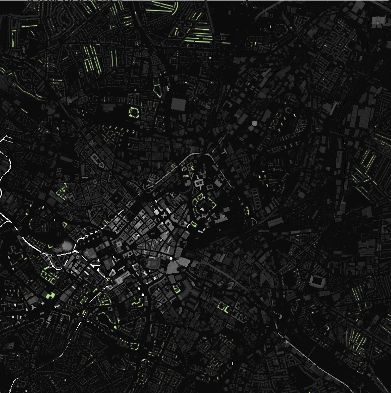
The shading is typically cast by other taller buildings or vegetation. With the DSM layer, we can get a reasonably accurate idea of the amount of shade cast onto a roof (at least accurate to a year ago). Without the DSM, we can still create a pseudo-DSM layer from the building height information.
Pseudo-DSM
Without a DSM, you can still compute the shading as long as you have the building height values and footprint for the surrounding buildings. To create the pseudo-DSM, rasterise the vector layer with the building height as the pixel value and leave all other pixels as ‘0’.
It will not be as accurate because our data only contains the heights for residential buildings and not all buildings. It also does not consider the height of vegetation.
UMEP: Solar Radiation: Shadow Generator
UMEP (Urban Multi-scale Universal Predictor) is an open-source climate service tool available as a plugin on QGIS. The Shadow Generator creates a model of the shadows produced at different times of the day and year from a DSM. However, it is a computationally expensive process. For scale, it takes 1 hour and 15 minutes to calculate the average shading of a 500 pixel by 500 pixel DSM over two days at two-hour intervals.
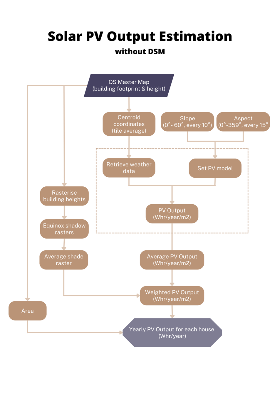
The final solar panel output requires all this information and details about the type of solar module being used to account for the efficiency and capacity of different systems.
pvlib is a Python library for simulating the performance of photovoltaic energy systems. There are many options for different modules you can use. The model also takes meteorological data from PVGIS based on coordinates and factors in the solar panel module’s slope, aspect and elevation.
If the roof slope and aspect are not available, you can calculate the solar panel output for several acceptable combinations of slopes (0°-60°, every 10°) and aspect (0°-359°, every 10°). Then, we will take the average output as the solar PV output for the house.
The output is the potential solar PV output in kWhr/year/m2.
I compared my estimates to the formula and final calculations from MCS and found that my results were within the same order of magnitude. However, there is no way to know for sure how accurate each estimation is without ground truth data.

‘Can we trust these results?’ is one of the most important questions to ask in data science. Your results are only as good as their reliability!
LIDAR data is fairly accurate (depending on your data source), and with buildings, a resolution of 1m is good enough for the level of granularity we are looking for. But if you are extending this method to smaller structures, you will need to proceed with caution. You should also double-check when the LIDAR data was last updated so it lines up with your building data.
Building footprint data depends on your source. Who collected the data? Open Street Map is an aggregation of open-source data and logs populated by people. Whereas government sources might have a more rigorous data collection method which you should check for soundness. Some questions to ask the data:
- When was the data last updated?
- Who collected the data? Were multiple parties involved and if so how did they ensure standardisation across data collection?
- Were any checks involved in ensuring the data is reliable?
- Which houses might have been left out from data collection? Which houses are more prone to error than others? How might some houses have been generalised?
The calculations run on QGIS are a reflection of the data’s reliability. There could be outliers if your LIDAR data doesn’t line up with your building footprint data. For example, a building could have been built after the LIDAR data was collected.
Perhaps the caveats I’ve left for the solar output estimations have left you pessimistic. What’s the point if I can’t validate it? Is this even worth doing?
My hope is that this methodology will pave the way for investments in building the appropriate validation data required to propel any future methods developed for solar panel estimation! All local councils and climate-focused organisations need data like this to help increase our renewable energy usage share and perhaps this will show you that this is worth investing in.
Mapping Solar PV Potential in Ambleside by Alex Boyd
QGIS
Building Footprint
LIDAR
A comprehensive guide for what it takes to estimate solar panel output using Python and QGIS
To figure out how much solar energy a rooftop can produce, we need the following information:
- Roof slope
- Roof azimuth (orientation towards the Sun)
- Number of solar panels a roof can hold
- Shading factor (the percentage of light that is blocked from shadows)
- Solar irradiance (how much total sunlight the roof receives)
The problem is that determining the first four variables requires a site visit which makes it more difficult to implement schemes or policies for installing solar panels. Instead, we can use publicly available data* to derive these variables to determine which areas have the potential for high solar panel output. Then, we can use different calculations to estimate the annual solar panel output for each rooftop.
* The extensiveness of data availabiltiy depends on the region of interest.
This article is an abstracted, generalised version of the methodology I applied at DSSGxUK for the West Midlands Combined Authority and Pure Leapfrog. See the GitHub repository for the full code and West Midlands (UK)-specific tutorial.
How much can we trust this methodology?
We need validation data to verify (1) the derived inputs and (2) the final solar panel output. The difficulty is procuring it.
You can sample Google Streetview images of houses to determine the roof slope and azimuth, and the number of solar panels the roof can hold(though this process will be tedious) or if you are lucky there might be a collected database. Though to be transparent, I haven’t found one myself.
Real validation data for solar panel output requires meter readings from installed solar panels or gathering the data yourself by fixing meters on a random set of rooftops to gauge the effect of shading on roofs.
Otherwise, you will have to rely on estimations from organisations such as the UK’s Microgeneration Certification Scheme Service (MCS) for comparison. Essentially, you’d simply be comparing different forms of estimation without any ground truth data. However, these can still serve as good ballpark estimates, so you know your estimations are at least within the correct order of magnitude.
You will need four pieces of data:
- Digital Surface Model (DSM): information on the elevation of the Earth’s surface including man-made structures (eg: buildings, bridges) and natural features (eg: trees, grass).
- Digital Terrain Model (DTM): information on the elevation of the Earth’s surface when it is bare of all natural and man-made structures. It still includes terrain features like rivers and hills.
- Building Footprint: information on the location of buildings represented by a polygon for each building.
- Solar Irradiance: the amount of solar power received in an area.
The availability of this data is subject to the area you are looking at. Some governments and open-source projects collect and publicly release this data. Some lie behind a paywall. In this article, I will share sources which provide global data and UK-specific sources I’ve found (since my project was focused on the West Midlands). These sources are non-exhaustive, so if you find others please leave a comment!
For now, I’ll explain what all this data is.
DSM and DTM from LIDAR data
If you are familiar with how echolocation (used by whales and dolphins) works, LIDAR works somewhat similarly. An aircraft flying at a fixed altitude will send out pulses of lasers (high-frequency light). The lasers reflect on surfaces and the time it takes for the lasers to return provides the distance (read here for more details).
The highest resolution I’ve seen for UK data is 25cm (only for a very small portion of the country) while resolutions of 1m and 2m cover almost everything. The resolution means that every pixel represents 25cm of space which makes for a clearer image.
LiDAR is just one method of measuring elevation. Researchers use this data to derive the DSM and DTM. You could also use satellite imaging or 3D models, but those are usually harder to find open-source and requires more processing power for the same level of granularity.
Building Footprint from Open Street Map
Building footprints help identify the shapes you see in the DSM and DTM and come in the form of shapefiles. Shapefiles are a type of vectorised file that stores the information about a geographic attribute (eg: coordinates, coordinate reference system, tag).
While some shapefiles are more accessible than others, you can turn to open data sources like Open Street Map to download the data too. They also have an API, check the resources to learn how to use them.
Check the government website of your region of interest! They will have building footprint data because they use it for city planning, it is a question of whether the data is publicly available. For example, Ordinance Survey only releases the centroids of buildings while the building footprint data is licensed.
Solar Irradiance Data
Solar irradiance is the sun of energy received from:
- Direct Normal Irradiance: the amount of sun rays a surface receives perpendicularly
- Diffuse Horizontal Irradiation: the sun rays that don’t reach the solar module perpendicularly
The maximum solar irradiance is achieved when the solar panel is under a clear sky, tilted equal to the latitude and facing South. You can get more detailed explanations here.
The EU JRC PVGIS online tool is a reliable resource for solar irradiance data. Other meteorological agencies will also have this data, but EU JRC PVGIS integrates well with one of the estimation methods I will introduce below.
Instead of looking at the roof as a single unit, it is more accurate to see it as a collection of segments which have their own azimuth (aspect) and slope.
The following methodology is adapted from Mapping Solar PV Potential in Ambleside. Our method only requires the DSM layer and building footprints, while the cited paper additionally requires the DTM layer to filter for height. I didn’t require a DTM because I had data on the building heights, but in the absence of this, you can use a DTM to supplement that data. Essentially, you can find the difference between the DSM and DTM layer to get the building heights.
The roof segmentation results are dubious even in the paper itself. The roof segments do not look like the segments you would draw yourself (Figure 4). The author only used a test set of 20 rooftops to get accuracy for slope and aspect within 10 degrees for 75% and 70% of the houses, respectively. These results leave much to be desired, and the poor roof segmentation indicates some of the author’s future work recommendations.
The shading is typically cast by other taller buildings or vegetation. With the DSM layer, we can get a reasonably accurate idea of the amount of shade cast onto a roof (at least accurate to a year ago). Without the DSM, we can still create a pseudo-DSM layer from the building height information.
Pseudo-DSM
Without a DSM, you can still compute the shading as long as you have the building height values and footprint for the surrounding buildings. To create the pseudo-DSM, rasterise the vector layer with the building height as the pixel value and leave all other pixels as ‘0’.
It will not be as accurate because our data only contains the heights for residential buildings and not all buildings. It also does not consider the height of vegetation.
UMEP: Solar Radiation: Shadow Generator
UMEP (Urban Multi-scale Universal Predictor) is an open-source climate service tool available as a plugin on QGIS. The Shadow Generator creates a model of the shadows produced at different times of the day and year from a DSM. However, it is a computationally expensive process. For scale, it takes 1 hour and 15 minutes to calculate the average shading of a 500 pixel by 500 pixel DSM over two days at two-hour intervals.
The final solar panel output requires all this information and details about the type of solar module being used to account for the efficiency and capacity of different systems.
pvlib is a Python library for simulating the performance of photovoltaic energy systems. There are many options for different modules you can use. The model also takes meteorological data from PVGIS based on coordinates and factors in the solar panel module’s slope, aspect and elevation.
If the roof slope and aspect are not available, you can calculate the solar panel output for several acceptable combinations of slopes (0°-60°, every 10°) and aspect (0°-359°, every 10°). Then, we will take the average output as the solar PV output for the house.
The output is the potential solar PV output in kWhr/year/m2.
I compared my estimates to the formula and final calculations from MCS and found that my results were within the same order of magnitude. However, there is no way to know for sure how accurate each estimation is without ground truth data.
‘Can we trust these results?’ is one of the most important questions to ask in data science. Your results are only as good as their reliability!
LIDAR data is fairly accurate (depending on your data source), and with buildings, a resolution of 1m is good enough for the level of granularity we are looking for. But if you are extending this method to smaller structures, you will need to proceed with caution. You should also double-check when the LIDAR data was last updated so it lines up with your building data.
Building footprint data depends on your source. Who collected the data? Open Street Map is an aggregation of open-source data and logs populated by people. Whereas government sources might have a more rigorous data collection method which you should check for soundness. Some questions to ask the data:
- When was the data last updated?
- Who collected the data? Were multiple parties involved and if so how did they ensure standardisation across data collection?
- Were any checks involved in ensuring the data is reliable?
- Which houses might have been left out from data collection? Which houses are more prone to error than others? How might some houses have been generalised?
The calculations run on QGIS are a reflection of the data’s reliability. There could be outliers if your LIDAR data doesn’t line up with your building footprint data. For example, a building could have been built after the LIDAR data was collected.
Perhaps the caveats I’ve left for the solar output estimations have left you pessimistic. What’s the point if I can’t validate it? Is this even worth doing?
My hope is that this methodology will pave the way for investments in building the appropriate validation data required to propel any future methods developed for solar panel estimation! All local councils and climate-focused organisations need data like this to help increase our renewable energy usage share and perhaps this will show you that this is worth investing in.
Mapping Solar PV Potential in Ambleside by Alex Boyd
QGIS
Building Footprint
LIDAR
Denial of responsibility! Techno Blender is an automatic aggregator of the all world’s media. In each content, the hyperlink to the primary source is specified. All trademarks belong to their rightful owners, all materials to their authors. If you are the owner of the content and do not want us to publish your materials, please contact us by email – [email protected]. The content will be deleted within 24 hours.