
Evaluating Synthetic Data — The Million Dollar Question
Evaluating Synthetic Data — The Million Dollar Question
Are my real and synthetic datasets random samples from the same parent distribution?
When we perform synthetic data generation, we typically create a model for our real (or ‘observed’) data, and then use this model to generate synthetic data. This observed data is usually compiled from real world experiences, such as measurements of the physical characteristics of irises or details about individuals who have defaulted on credit or acquired some medical condition. We can think of the observed data as having come from some ‘parent distribution’ — the true underlying distribution from which the observed data is a random sample. Of course, we never know this parent distribution — it must be estimated, and this is the purpose of our model.
But if our model can produce synthetic data that can be considered to be a random sample from the same parent distribution, then we’ve hit the jackpot: the synthetic data will possess the same statistical properties and patterns as the observed data (fidelity); it will be just as useful when put to tasks such as regression or classification (utility); and, because it is a random sample, there is no risk of it identifying the observed data (privacy). But how can we know if we have met this elusive goal?
In the first part of this story, we will conduct some simple experiments to gain a better understanding of the problem and motivate a solution. In the second part we will evaluate performance of a variety of synthetic data generators on a collection of well-known datasets.
Part 1 — Some Simple Experiments
Consider the following two datasets and try to answer this question:
Are the datasets random samples from the same parent distribution, or has one been derived from the other by applying small random perturbations?

The datasets clearly display similar statistical properties, such as marginal distributions and covariances. They would also perform similarly on a classification task in which a classifier trained on one dataset is tested on the other. So, fidelity and utility alone are inconclusive.
But suppose we were to plot the data points from each dataset on the same graph. If the datasets are random samples from the same parent distribution, we would intuitively expect the points from one dataset to be interspersed with those from the other in such a manner that, on average, points from one set are as close to — or ‘as similar to’ — their closest neighbors in that set as they are to their closest neighbors in the other set. However, if one dataset is a slight random perturbation of the other, then points from one set will be more similar to their closest neighbors in the other set than they are to their closest neighbors in the same set. This leads to the following test.
The Maximum Similarity Test
For each dataset, calculate the similarity between each instance and its closest neighbor in the same dataset. Call these the ‘maximum intra-set similarities’. If the datasets have the same distributional characteristics, then the distribution of intra-set similarities should be similar for each dataset. Now calculate the similarity between each instance of one dataset and its closest neighbor in the other dataset and call these the ‘maximum cross-set similarities’. If the distribution of maximum cross-set similarities is the same as the distribution of maximum intra-set similarities, then the datasets can be considered random samples from the same parent distribution. For the test to be valid, each dataset should contain the same number of examples.
Since the datasets we deal with in this story all contain a mixture of numerical and categorical variables, we need a similarity measure which can accommodate this. We use Gower Similarity¹.
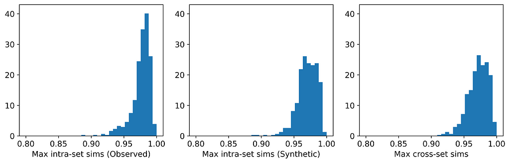
The table and histograms below show the means and distributions of the maximum intra- and cross-set similarities for Datasets 1 and 2.

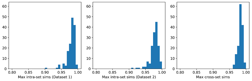
On average, the instances in one data set are more similar to their closest neighbors in the other dataset than they are to their closest neighbors in the same dataset. This indicates that the datasets are more likely to be perturbations of each other than random samples from the same parent distribution. And indeed, they are perturbations! Dataset 1 was generated from a Gaussian mixture model; Dataset 2 was generated by selecting (without replacement) an instance from Dataset 1 and applying a small random perturbation.
Ultimately, we will be using the Maximum Similarity Test to compare synthetic datasets with observed datasets. The biggest danger with synthetic data points being too close to observed points is privacy; i.e., being able to identify points in the observed set from points in the synthetic set. In fact, if you examine Datasets 1 and 2 carefully, you might actually be able to identify some such pairs. And this is for a case in which the average maximum cross-set similarity is only 0.3% larger than the average maximum intra-set similarity!
Modeling and Synthesizing
To end this first part of the story, let’s create a model for a dataset and use the model to generate synthetic data. We can then use the Maximum Similarity Test to compare the synthetic and observed sets.
The dataset on the left in the figure below is just Dataset 1 from above. The dataset on the right (Dataset 3) is the synthetic dataset. (We have estimated the distribution as a Gaussian mixture, but that’s not important).
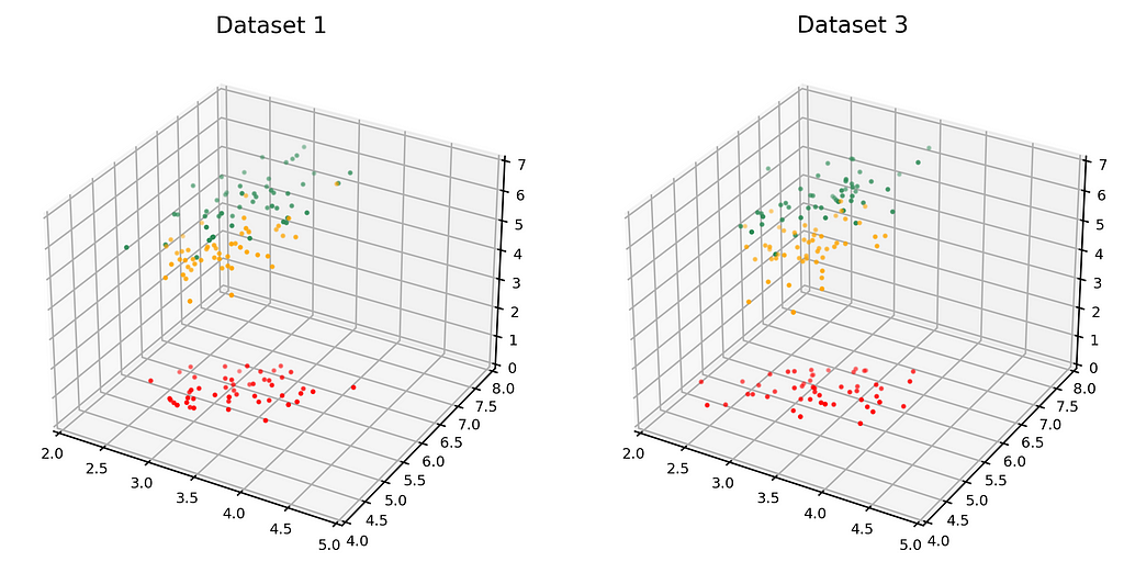
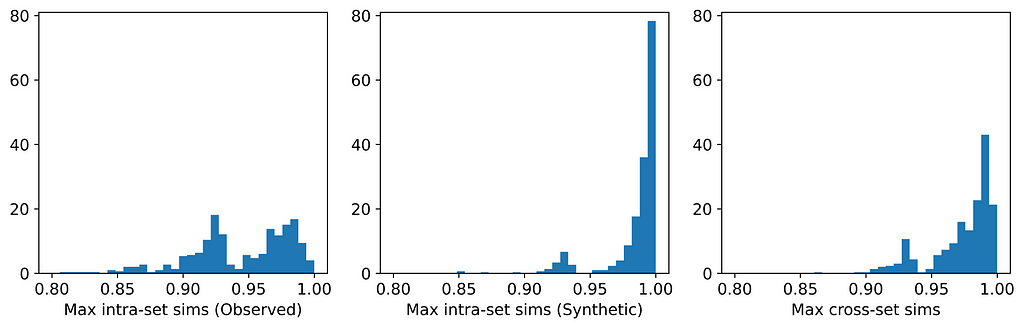
Here are the average similarities and histograms:

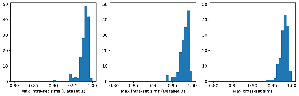
The three averages are identical to three significant figures, and the three histograms are very similar. Therefore, according to the Maximum Similarity Test, both datasets can reasonably be considered random samples from the same parent distribution. Our synthetic data generation exercise has been a success, and we have achieved the hat-trick — fidelity, utility, and privacy.
[Python code used to produce the datasets, plots and histograms from Part 1 is available from https://github.com/a-skabar/TDS-EvalSynthData]
Part 2— Real Datasets, Real Generators
The dataset used in Part 1 is simple and can be easily modeled with just a mixture of Gaussians. However, most real-world datasets are far more complex. In this part of the story, we will apply several synthetic data generators to some popular real-world datasets. Our primary focus is on comparing the distributions of maximum similarities within and between the observed and synthetic datasets to understand the extent to which they can be considered random samples from the same parent distribution.
The six datasets originate from the UCI repository² and are all popular datasets that have been widely used in the machine learning literature for decades. All are mixed-type datasets, and were chosen because they vary in their balance of categorical and numerical features.
The six generators are representative of the major approaches used in synthetic data generation: copula-based, GAN-based, VAE-based, and approaches using sequential imputation. CopulaGAN³, GaussianCopula, CTGAN³ and TVAE³ are all available from the Synthetic Data Vault libraries⁴, synthpop⁵ is available as an open-source R package, and ‘UNCRi’ refers to the synthetic data generation tool developed under the proprietary Unified Numeric/Categorical Representation and Inference (UNCRi) framework⁶. All generators were used with their default settings.
The table below shows the average maximum intra- and cross-set similarities for each generator applied to each dataset. Entries highlighted in red are those in which privacy has been compromised (i.e., the average maximum cross-set similarity exceeds the average maximum intra-set similarity on the observed data). Entries highlighted in green are those with the highest average maximum cross-set similarity (not including those in red). The last column shows the result of performing a Train on Synthetic, Test on Real (TSTR) test, where a classifier or regressor is trained on the synthetic examples and tested on the real (observed) examples. The Boston Housing dataset is a regression task, and the mean absolute error (MAE) is reported; all other tasks are classification tasks, and the reported value is the area under ROC curve (AUC).

The figures below display, for each dataset, the distributions of maximum intra- and cross-set similarities corresponding to the generator that attained the highest average maximum cross-set similarity (excluding those highlighted in red above).

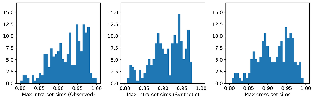
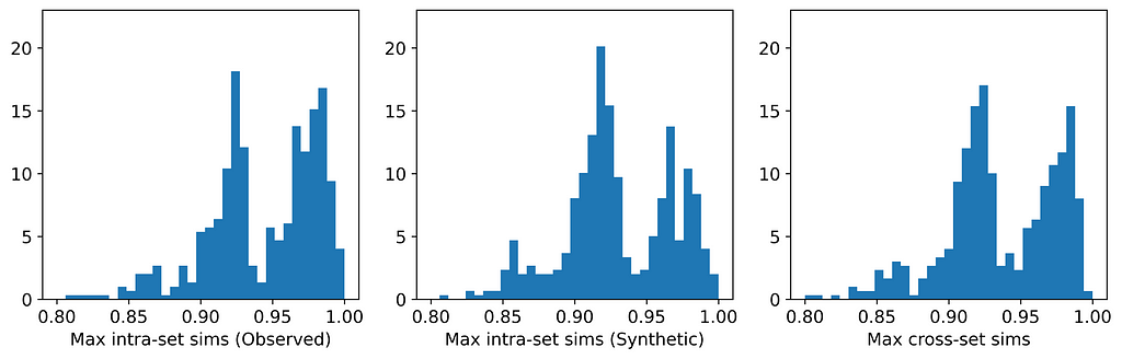

From the table, we can see that for those generators that did not breach privacy, the average maximum cross-set similarity is very close to the average maximum intra-set similarity on observed data. The histograms show us the distributions of these maximum similarities, and we can see that in most cases the distributions are clearly similar — strikingly so for datasets such as the Census Income dataset. The table also shows that the generator that achieved the highest average maximum cross-set similarity for each dataset (excluding those highlighted in red) also demonstrated best performance on the TSTR test (again excluding those in red). Thus, while we can never claim to have discovered the ‘true’ underlying distribution, these results demonstrate that the most effective generator for each dataset has captured the crucial features of the underlying distribution.
Privacy
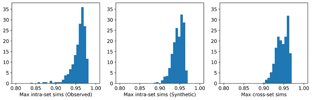
Only two of the seven generators displayed issues with privacy: synthpop and TVAE. Each of these breached privacy on three out of the six datasets. In two instances, specifically TVAE on Cleveland Heart Disease and TVAE on Credit Approval, the breach was particularly severe. The histograms for TVAE on Credit Approval are shown below and demonstrate that the synthetic examples are far too similar to each other, and also to their closest neighbors in the observed data. The model is a particularly poor representation of the underlying parent distribution. The reason for this may be that the Credit Approval dataset contains several numerical features that are extremely highly skewed.
Other observations and comments
The two GAN-based generators — CopulaGAN and CTGAN — were consistently among the worst performing generators. This was somewhat surprising given the immense popularity of GANs.
The performance of GaussianCopula was mediocre on all datasets except Wisconsin Breast Cancer, for which it attained the equal-highest average maximum cross-set similarity. Its unimpressive performance on the Iris dataset was particularly surprising, given that this is a very simple dataset that can easily be modeled using a mixture of Gaussians, and which we expected would be well-matched to Copula-based methods.
The generators which perform most consistently well across all datasets are synthpop and UNCRi, which both operate by sequential imputation. This means that they only ever need to estimate and sample from a univariate conditional distribution (e.g., P(x₇|x₁, x₂, …)), and this is typically much easier than modeling and sampling from a multivariate distribution (e.g., P(x₁, x₂, x₃, …)), which is (implicitly) what GANs and VAEs do. Whereas synthpop estimates distributions using decision trees (which are the source of the overfitting that synthpop is prone to), the UNCRi generator estimates distributions using a nearest neighbor-based approach, with hyper-parameters optimized using a cross-validation procedure that prevents overfitting.
Conclusion
Synthetic data generation is a new and evolving field, and while there are still no standard evaluation techniques, there is consensus that tests should cover fidelity, utility and privacy. But while each of these is important, they are not on an equal footing. For example, a synthetic dataset may achieve good performance on fidelity and utility but fail on privacy. This does not give it a ‘two out of three’: if the synthetic examples are too close to the observed examples (thus failing the privacy test), the model has been overfitted, rendering the fidelity and utility tests meaningless. There has been a tendency among some vendors of synthetic data generation software to propose single-score measures of performance that combine results from a multitude of tests. This is essentially based on the same ‘two out of three’ logic.
If a synthetic dataset can be considered a random sample from the same parent distribution as the observed data, then we cannot do any better — we have achieved maximum fidelity, utility and privacy. The Maximum Similarity Test provides a measure of the extent to which two datasets can be considered random samples from the same parent distribution. It is based on the simple and intuitive notion that if an observed and a synthetic dataset are random samples from the same parent distribution, instances should be distributed such that a synthetic instance is as similar on average to its closest observed instance as an observed instance is similar on average to its closest observed instance.
We propose the following single-score measure of synthetic dataset quality:

The closer this ratio is to 1 — without exceeding 1 — the better the quality of the synthetic data. It should, of course, be accompanied by a sanity check of the histograms.
References
[1] Gower, J. C. (1971). A general coefficient of similarity and some of its properties. Biometrics, 27(4), 857–871.
[2] Dua, D. & Graff, C., (2017). UCI Machine Learning Repository, Available at: http://archive.ics.uci.edu/ml.
[3] Xu, L., Skoularidou, M., Cuesta-Infante, A. and Veeramachaneni., K. Modeling Tabular data using Conditional GAN. NeurIPS, 2019.
[4] Patki, N., Wedge, R., & Veeramachaneni, K. (2016). The synthetic data vault. In 2016 IEEE International Conference on Data Science and Advanced Analytics (DSAA) (pp. 399–410). IEEE.
[5] Nowok, B., Raab G.M., Dibben, C. (2016). “synthpop: Bespoke Creation of Synthetic Data in R.” Journal of Statistical Software, 74(11), 1–26. doi:10.18637/jss.v074.i11.
[6] http://skanalytix.com/uncri-framework
[7] Harrison, D., & Rubinfeld, D.L. (1978). Boston Housing Dataset. Kaggle. https://www.kaggle.com/c/boston-housing. Licensed for commercial use under the CC: Public Domain license.
[8] Kohavi, R. (1996). Census Income. UCI Machine Learning Repository. https://doi.org/10.24432/C5GP7S. Licensed for commercial use under a Creative Commons Attribution 4.0 International (CC BY 4.0) license.
[9] Janosi, A., Steinbrunn, W., Pfisterer, M. and Detrano, R. (1988). Heart Disease. UCI Machine Learning Repository. https://doi.org/10.24432/C52P4X. Licensed for commercial use under a Creative Commons Attribution 4.0 International (CC BY 4.0) license.
[10] Quinlan, J.R. (1987). Credit Approval. UCI Machine Learning Repository. https://doi.org/10.24432/C5FS30. Licensed for commercial use under a Creative Commons Attribution 4.0 International (CC BY 4.0) license.
[11] Fisher, R.A. (1988). Iris. UCI Machine Learning Repository. https://doi.org/10.24432/C56C76. Licensed for commercial use under a Creative Commons Attribution 4.0 International (CC BY 4.0) license.
[12] Wolberg, W., Mangasarian, O., Street, N. and Street,W. (1995). Breast Cancer Wisconsin (Diagnostic). UCI Machine Learning Repository. https://doi.org/10.24432/C5DW2B. Licensed for commercial use under a Creative Commons Attribution 4.0 International (CC BY 4.0) license.
Evaluating Synthetic Data — The Million Dollar Question was originally published in Towards Data Science on Medium, where people are continuing the conversation by highlighting and responding to this story.
Evaluating Synthetic Data — The Million Dollar Question
Are my real and synthetic datasets random samples from the same parent distribution?

When we perform synthetic data generation, we typically create a model for our real (or ‘observed’) data, and then use this model to generate synthetic data. This observed data is usually compiled from real world experiences, such as measurements of the physical characteristics of irises or details about individuals who have defaulted on credit or acquired some medical condition. We can think of the observed data as having come from some ‘parent distribution’ — the true underlying distribution from which the observed data is a random sample. Of course, we never know this parent distribution — it must be estimated, and this is the purpose of our model.
But if our model can produce synthetic data that can be considered to be a random sample from the same parent distribution, then we’ve hit the jackpot: the synthetic data will possess the same statistical properties and patterns as the observed data (fidelity); it will be just as useful when put to tasks such as regression or classification (utility); and, because it is a random sample, there is no risk of it identifying the observed data (privacy). But how can we know if we have met this elusive goal?
In the first part of this story, we will conduct some simple experiments to gain a better understanding of the problem and motivate a solution. In the second part we will evaluate performance of a variety of synthetic data generators on a collection of well-known datasets.
Part 1 — Some Simple Experiments
Consider the following two datasets and try to answer this question:
Are the datasets random samples from the same parent distribution, or has one been derived from the other by applying small random perturbations?
The datasets clearly display similar statistical properties, such as marginal distributions and covariances. They would also perform similarly on a classification task in which a classifier trained on one dataset is tested on the other. So, fidelity and utility alone are inconclusive.
But suppose we were to plot the data points from each dataset on the same graph. If the datasets are random samples from the same parent distribution, we would intuitively expect the points from one dataset to be interspersed with those from the other in such a manner that, on average, points from one set are as close to — or ‘as similar to’ — their closest neighbors in that set as they are to their closest neighbors in the other set. However, if one dataset is a slight random perturbation of the other, then points from one set will be more similar to their closest neighbors in the other set than they are to their closest neighbors in the same set. This leads to the following test.
The Maximum Similarity Test
For each dataset, calculate the similarity between each instance and its closest neighbor in the same dataset. Call these the ‘maximum intra-set similarities’. If the datasets have the same distributional characteristics, then the distribution of intra-set similarities should be similar for each dataset. Now calculate the similarity between each instance of one dataset and its closest neighbor in the other dataset and call these the ‘maximum cross-set similarities’. If the distribution of maximum cross-set similarities is the same as the distribution of maximum intra-set similarities, then the datasets can be considered random samples from the same parent distribution. For the test to be valid, each dataset should contain the same number of examples.
Since the datasets we deal with in this story all contain a mixture of numerical and categorical variables, we need a similarity measure which can accommodate this. We use Gower Similarity¹.
The table and histograms below show the means and distributions of the maximum intra- and cross-set similarities for Datasets 1 and 2.
On average, the instances in one data set are more similar to their closest neighbors in the other dataset than they are to their closest neighbors in the same dataset. This indicates that the datasets are more likely to be perturbations of each other than random samples from the same parent distribution. And indeed, they are perturbations! Dataset 1 was generated from a Gaussian mixture model; Dataset 2 was generated by selecting (without replacement) an instance from Dataset 1 and applying a small random perturbation.
Ultimately, we will be using the Maximum Similarity Test to compare synthetic datasets with observed datasets. The biggest danger with synthetic data points being too close to observed points is privacy; i.e., being able to identify points in the observed set from points in the synthetic set. In fact, if you examine Datasets 1 and 2 carefully, you might actually be able to identify some such pairs. And this is for a case in which the average maximum cross-set similarity is only 0.3% larger than the average maximum intra-set similarity!
Modeling and Synthesizing
To end this first part of the story, let’s create a model for a dataset and use the model to generate synthetic data. We can then use the Maximum Similarity Test to compare the synthetic and observed sets.
The dataset on the left in the figure below is just Dataset 1 from above. The dataset on the right (Dataset 3) is the synthetic dataset. (We have estimated the distribution as a Gaussian mixture, but that’s not important).
Here are the average similarities and histograms:
The three averages are identical to three significant figures, and the three histograms are very similar. Therefore, according to the Maximum Similarity Test, both datasets can reasonably be considered random samples from the same parent distribution. Our synthetic data generation exercise has been a success, and we have achieved the hat-trick — fidelity, utility, and privacy.
[Python code used to produce the datasets, plots and histograms from Part 1 is available from https://github.com/a-skabar/TDS-EvalSynthData]
Part 2— Real Datasets, Real Generators
The dataset used in Part 1 is simple and can be easily modeled with just a mixture of Gaussians. However, most real-world datasets are far more complex. In this part of the story, we will apply several synthetic data generators to some popular real-world datasets. Our primary focus is on comparing the distributions of maximum similarities within and between the observed and synthetic datasets to understand the extent to which they can be considered random samples from the same parent distribution.
The six datasets originate from the UCI repository² and are all popular datasets that have been widely used in the machine learning literature for decades. All are mixed-type datasets, and were chosen because they vary in their balance of categorical and numerical features.
The six generators are representative of the major approaches used in synthetic data generation: copula-based, GAN-based, VAE-based, and approaches using sequential imputation. CopulaGAN³, GaussianCopula, CTGAN³ and TVAE³ are all available from the Synthetic Data Vault libraries⁴, synthpop⁵ is available as an open-source R package, and ‘UNCRi’ refers to the synthetic data generation tool developed under the proprietary Unified Numeric/Categorical Representation and Inference (UNCRi) framework⁶. All generators were used with their default settings.
The table below shows the average maximum intra- and cross-set similarities for each generator applied to each dataset. Entries highlighted in red are those in which privacy has been compromised (i.e., the average maximum cross-set similarity exceeds the average maximum intra-set similarity on the observed data). Entries highlighted in green are those with the highest average maximum cross-set similarity (not including those in red). The last column shows the result of performing a Train on Synthetic, Test on Real (TSTR) test, where a classifier or regressor is trained on the synthetic examples and tested on the real (observed) examples. The Boston Housing dataset is a regression task, and the mean absolute error (MAE) is reported; all other tasks are classification tasks, and the reported value is the area under ROC curve (AUC).
The figures below display, for each dataset, the distributions of maximum intra- and cross-set similarities corresponding to the generator that attained the highest average maximum cross-set similarity (excluding those highlighted in red above).
From the table, we can see that for those generators that did not breach privacy, the average maximum cross-set similarity is very close to the average maximum intra-set similarity on observed data. The histograms show us the distributions of these maximum similarities, and we can see that in most cases the distributions are clearly similar — strikingly so for datasets such as the Census Income dataset. The table also shows that the generator that achieved the highest average maximum cross-set similarity for each dataset (excluding those highlighted in red) also demonstrated best performance on the TSTR test (again excluding those in red). Thus, while we can never claim to have discovered the ‘true’ underlying distribution, these results demonstrate that the most effective generator for each dataset has captured the crucial features of the underlying distribution.
Privacy
Only two of the seven generators displayed issues with privacy: synthpop and TVAE. Each of these breached privacy on three out of the six datasets. In two instances, specifically TVAE on Cleveland Heart Disease and TVAE on Credit Approval, the breach was particularly severe. The histograms for TVAE on Credit Approval are shown below and demonstrate that the synthetic examples are far too similar to each other, and also to their closest neighbors in the observed data. The model is a particularly poor representation of the underlying parent distribution. The reason for this may be that the Credit Approval dataset contains several numerical features that are extremely highly skewed.
Other observations and comments
The two GAN-based generators — CopulaGAN and CTGAN — were consistently among the worst performing generators. This was somewhat surprising given the immense popularity of GANs.
The performance of GaussianCopula was mediocre on all datasets except Wisconsin Breast Cancer, for which it attained the equal-highest average maximum cross-set similarity. Its unimpressive performance on the Iris dataset was particularly surprising, given that this is a very simple dataset that can easily be modeled using a mixture of Gaussians, and which we expected would be well-matched to Copula-based methods.
The generators which perform most consistently well across all datasets are synthpop and UNCRi, which both operate by sequential imputation. This means that they only ever need to estimate and sample from a univariate conditional distribution (e.g., P(x₇|x₁, x₂, …)), and this is typically much easier than modeling and sampling from a multivariate distribution (e.g., P(x₁, x₂, x₃, …)), which is (implicitly) what GANs and VAEs do. Whereas synthpop estimates distributions using decision trees (which are the source of the overfitting that synthpop is prone to), the UNCRi generator estimates distributions using a nearest neighbor-based approach, with hyper-parameters optimized using a cross-validation procedure that prevents overfitting.
Conclusion
Synthetic data generation is a new and evolving field, and while there are still no standard evaluation techniques, there is consensus that tests should cover fidelity, utility and privacy. But while each of these is important, they are not on an equal footing. For example, a synthetic dataset may achieve good performance on fidelity and utility but fail on privacy. This does not give it a ‘two out of three’: if the synthetic examples are too close to the observed examples (thus failing the privacy test), the model has been overfitted, rendering the fidelity and utility tests meaningless. There has been a tendency among some vendors of synthetic data generation software to propose single-score measures of performance that combine results from a multitude of tests. This is essentially based on the same ‘two out of three’ logic.
If a synthetic dataset can be considered a random sample from the same parent distribution as the observed data, then we cannot do any better — we have achieved maximum fidelity, utility and privacy. The Maximum Similarity Test provides a measure of the extent to which two datasets can be considered random samples from the same parent distribution. It is based on the simple and intuitive notion that if an observed and a synthetic dataset are random samples from the same parent distribution, instances should be distributed such that a synthetic instance is as similar on average to its closest observed instance as an observed instance is similar on average to its closest observed instance.
We propose the following single-score measure of synthetic dataset quality:
The closer this ratio is to 1 — without exceeding 1 — the better the quality of the synthetic data. It should, of course, be accompanied by a sanity check of the histograms.
References
[1] Gower, J. C. (1971). A general coefficient of similarity and some of its properties. Biometrics, 27(4), 857–871.
[2] Dua, D. & Graff, C., (2017). UCI Machine Learning Repository, Available at: http://archive.ics.uci.edu/ml.
[3] Xu, L., Skoularidou, M., Cuesta-Infante, A. and Veeramachaneni., K. Modeling Tabular data using Conditional GAN. NeurIPS, 2019.
[4] Patki, N., Wedge, R., & Veeramachaneni, K. (2016). The synthetic data vault. In 2016 IEEE International Conference on Data Science and Advanced Analytics (DSAA) (pp. 399–410). IEEE.
[5] Nowok, B., Raab G.M., Dibben, C. (2016). “synthpop: Bespoke Creation of Synthetic Data in R.” Journal of Statistical Software, 74(11), 1–26. doi:10.18637/jss.v074.i11.
[6] http://skanalytix.com/uncri-framework
[7] Harrison, D., & Rubinfeld, D.L. (1978). Boston Housing Dataset. Kaggle. https://www.kaggle.com/c/boston-housing. Licensed for commercial use under the CC: Public Domain license.
[8] Kohavi, R. (1996). Census Income. UCI Machine Learning Repository. https://doi.org/10.24432/C5GP7S. Licensed for commercial use under a Creative Commons Attribution 4.0 International (CC BY 4.0) license.
[9] Janosi, A., Steinbrunn, W., Pfisterer, M. and Detrano, R. (1988). Heart Disease. UCI Machine Learning Repository. https://doi.org/10.24432/C52P4X. Licensed for commercial use under a Creative Commons Attribution 4.0 International (CC BY 4.0) license.
[10] Quinlan, J.R. (1987). Credit Approval. UCI Machine Learning Repository. https://doi.org/10.24432/C5FS30. Licensed for commercial use under a Creative Commons Attribution 4.0 International (CC BY 4.0) license.
[11] Fisher, R.A. (1988). Iris. UCI Machine Learning Repository. https://doi.org/10.24432/C56C76. Licensed for commercial use under a Creative Commons Attribution 4.0 International (CC BY 4.0) license.
[12] Wolberg, W., Mangasarian, O., Street, N. and Street,W. (1995). Breast Cancer Wisconsin (Diagnostic). UCI Machine Learning Repository. https://doi.org/10.24432/C5DW2B. Licensed for commercial use under a Creative Commons Attribution 4.0 International (CC BY 4.0) license.
Evaluating Synthetic Data — The Million Dollar Question was originally published in Towards Data Science on Medium, where people are continuing the conversation by highlighting and responding to this story.
Denial of responsibility! Techno Blender is an automatic aggregator of the all world’s media. In each content, the hyperlink to the primary source is specified. All trademarks belong to their rightful owners, all materials to their authors. If you are the owner of the content and do not want us to publish your materials, please contact us by email – [email protected]. The content will be deleted within 24 hours.