
Exploration of Quantum Computing: Solving Optimisation Problem Using Quantum Annealer | by Ken Moriwaki | Jul, 2022
Catch up with the current state of quantum computing and experiment using quantum annealer as a service by D-Wave.
This article aims to overview quantum computing and explore quantum annealer, a specialised machine for solving combinatorial optimisation problems, through an example.
We go through the basic concepts behind quantum computing and understand two different types of quantum computers. Then, we focus on problem-solving practices with an example of portfolio optimisation using Python programming and quantum annealer as a service provided by D-Wave.
If you’d like to dive into the implementation, please feel free to skip sections to “Implementation Using Quantum Annealer”.
Moore’s law may be obsolete within a decade or two. We are challenged by the physical limit of the size of the transistor in silicon microchips. The advances in computing power may become slower than we have witnessed in the past 50 years. There are alternative solutions in pursuit of breaking through such barriers. For example, the use of the Graphical Processing Unit (GPU) and the development of the Tensor Processing Unit (TPU) has accelerated the processing speed in deep learning. One of the most exciting candidates that could cause a paradigm shift would be quantum computing (QC).
Figure 1 is Google’s search trend for “quantum computing” for the past five years, starting from July 2017. There was a moment when the term had a sudden spike. In October 2019, Google announced that they achieved quantum supremacy [1], i.e., their QC machine with quantum processing unit (QPU) outperformed the state-of-the-art “classical” supercomputer by 158 million times.
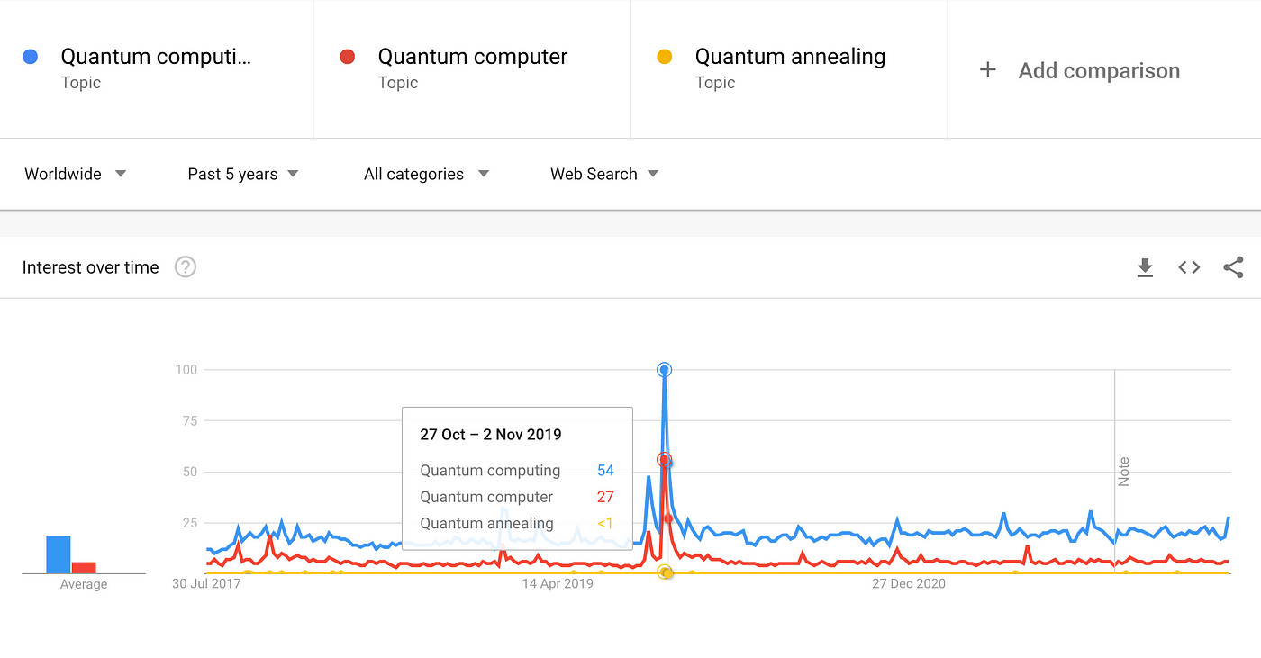
Though it attracted people’s attention, the interests of the general public failed to keep the momentum. It is often considered that QC is hype because it lacks applications for real-life problems. Professor Christopher Monroe, a famous American Physicist for his development of trapped ion quantum computers, described QC as “a marathon not a sprint” [2] which may explain the state of quantum technologies very well, but where is QC today?
Though we do not see any presence of quantum machines in our everyday life, the QC has become much closer to us than it was a decade ago. We can now easily access quantum resources via cloud services. In this article, we will experience QC as a service provided by D-Wave, whose machines are often used in academic and commercial research.
First, we will understand the basics of QC and two types of computing systems: gate model and quantum annealing. Then, we shift our focus to quantum annealing from theoretical and practical perspectives.
Quantum computers are machines that execute calculations using the characteristics of quantum mechanics, which is based on the mysterious nature of the microworld. “I think I can safely say that nobody understands quantum mechanics,” said Nobel laureate Physicist Richard Feynman [3]. What is occurring at the quantum scale follows the different laws of physics from what we know empirically.
A miracle is realised by a quantum bit (qubit) that can represent the dual state of 0 and 1 simultaneously, while a classic binary bit can only take either 0 or 1 at a time. This phenomenon is called superposition [4]. For example, to express two bit-combinations using the classical computer, we need 2² = 4 combinations, [00, 01, 10, 11], but two qubits can represent all four possible combinations simultaneously. Then, classical computers check each combination sequentially and then find a solution at most with four calculations. On the other hand, a quantum takes advantage of its wave nature so that the wave interference increases the probability of the desired state and decreases the other to reach a correct solution effectively all at once.
What are the qubits made of? They can be developed using different materials and principles. For example, IBM Quantum uses niobium and aluminium on a silicon base [5] to achieve superconductivity under near absolute zero temperature. ION Q in the USA uses “trapped ion quantum” from Ytterbium, a rare earth metal [6]. Another example is Xanadu in Canada applies photonics (light particles) in the quantum processing unit [7]. The use of ion and light has advantages over the superconductivity materials as it works under room temperature; the superconducting qubits are more scalable and implemented by other companies like Google [8] and D-Wave [9]. It is exciting to see future innovations in this area.
The concept of QC dates to the 1980s, but it was in the early 2010s when more and more people talked about it being the next big thing. However, it is not well-known what problems quantum computers can solve. We can classify quantum computers into “gate model” and “quantum annealing”. They have different use cases and architecture.
Gate Model
The quantum gate model computers are designed for universal purposes by applying gates to build complex algorithms. They can be considered the upward compatible machines of classical computers but exponentially fast if appropriate quantum algorithms like Shor [10] and Grover [11] are used. The applications include prime factorisation, which becomes a threat to the existing secure data transmission methods over the internet using RSA (Rivest–Shamir–Adleman) keys, quantum simulations which have the potential for finding new medicines, and machine learning. However, the gate model requires high-quality qubit processors; the number of qubits is limited to two digits (except for IBM’s exploratory 127-qubit Eagle system.)
Quantum Annealing
On the other hand, quantum annealers shine when they are used to search for the best from a vast number of possible combinations. Such challenges are called combinatorial optimisation problems. Many applications of quantum annealing have been reported recently [12]. There are also researches to develop novel machine learning algorithms using quantum annealers. In [13], Amin et al. showed that there were possibilities to use quantum annealing hardware as a sampler for Boltzmann Machine by exploiting its quantum nature.
In physics, the minimum energy principle states that the internal energy decreases and approaches the minimum values [14]. If we can formulate our problems in the form of an energy minimisation equation, the quantum annealer will be able to search for the best possible answer.
Quantum annealer is relatively noise-tolerant compared to the gate model [15]. At the time of this writing, the most considerable number of qubits on a quantum processing unit (QPU) is at least five thousand provided by D-Wave’s Advantage solver [16]. It is expected to increase more in the coming years. Five thousand qubits is a large number compared to what is achieved by the gate model. However, what we obtain from the annealer is as limited as a set of 5k-bit values per sampling. Furthermore, not all qubits are connected. Therefore, a hybrid system of classical computing and the quantum annealer is being developed to complement the capabilities of the two systems.
Annealing is a technique used to make quality iron products by heating the material to a certain degree of temperature and cooling it down slowly. The iron’s mechanical characteristics are altered through the heat treatment, which reduces the hardness and increases the elasticity [17].
Simulated annealing (SA) is a probabilistic technique whose name and idea are derived from annealing in material science. SA is a meta-heuristic in which algorithms approximate the global minimum or maximum of a given function. It uses a parameter called temperature that is initialised with a high value and decreases as the algorithm proceeds, like the physical annealing. High-temperature value promotes the algorithm to look for the various parts of the problem space, which helps to avoid being stuck in local minima or maxima. When the temperature goes down to zero, the state reaches the optimal point if successful. Going through the SA algorithm is outside the scope of this article, and the details on how it works can be found, for example, on the MathWorks website.
Quantum annealing (QA) is an algorithm to solve combinatorial optimisation problems mainly. Instead of using temperature to explore the problem space, QA uses the laws of quantum mechanics to measure the energy state. Starting from the qubits’ dual state, where all the possible combinations of the values are equally likely to happen, we can gradually reduce such quantum mechanical effects by the process called quantum fluctuation to reach the most optimal point where the lowest energy state is realised.
In [18], Kadowaki and Nishimori proved that QA converges to the optimal state with a much larger probability than SA in almost all cases on classical computers. The actual quantum annealing machines were developed by D-Wave and built on the ground of their theoretical framework.
QA machines are specialised hardware to solve combinatorial optimisation problems. These problems can be found in many places in our life. For example, an Amazon delivery person needs to find the most optimal route to deliver all parcels given for the day. The objective is to find a route with the shortest distance to visit all the delivery addresses. We can treat the distance as the energy in the QA context and find the path that reaches the ground state. We can also think of a futuristic example where multiple autonomous cars are navigated to optimise the traffic in a specific city area with heavy traffic jams. The objective is to reduce the traffic by minimising the number of overlaps of cars taking the same route simultaneously while each car aims to optimise the travel time to a destination. One prominet example of the traffic optimisation challenge conducted by researchers at the Volkswagen Group and D-Wave using quantum annealer can be found in [19].
Quantum annealers require an objective function to be defined in the Ising model or Quadratic Unconstrained Binary Optimisation (QUBO). Ising model is a mathematical model in statistical mechanics. QUBO is mathematically equivalent [20] to the Ising model and is much simpler to formulate a problem.
QUBO is a minimisation objective function expressed as follows:
where x_i and x_j {i,j =0,1,…,N} takes 0 or 1. Q_{ij} is a coefficient matrix of size n x n, which we need to prepare for a QA machine. In case of a problem to search for a global maximum, we can flip the sign to minus to convert the problem into a minimisation problem.
In reality, a problem must be satisfied with one or more constraints. For example, a knapsack problem has a constraint of how many weights you can pack things in the bag. Such constraints are multiplied by weight parameters and are added to the objective function as penalty terms.
In this section, we would like to code and solve a simple combinatorial optimisation problem in Python and the real Quantum Annealer by D-Wave.
Preparation
Before starting, we need to sign up for a cloud computing service. D-wave offers trial access to QA solvers with a sixty-second computational time allowance for one month. Please go to D-Wave Leap to find out more. After successful registration, the API token is available on the dashboard.
Problem Setting
In this article, we would like to challenge a simplified portfolio optimisation problem. Suppose there are twenty candidate stocks from FTSE100 to invest in. Our objective is to maximise an expected return rate at the minimum risk while keeping more or less ten stocks in our portfolio.
We will take the following five steps to solve the problem:
1. Import historical stock price data from the internet
2. Prepare data by cleansing and feature engineering
3. Formulate the cost functions and constraints to obtain a QUBO matrix
4. Sample optimisation results from a D-Wave solver
5. Sample optimisation results from a simulated quantum annealing solver
6. Evaluate the outcomes
Each of the above steps is demonstrated in a Colab notebook found in Python Coding in Colab Notebook section.
Dependencies
Some notes on the Python requirements:
- yfinance is used to retrieve stock price data from Yahoo! Finance.
- Prophet is a python package used to make time-series forecasting. It is possible to do multivariate time series forecasting and add holiday effects easily.
- D-Wave Ocean SDK needs to be installed. The SDK includes packages that are necessary to communicate with D-Wave resources.
- PyQUBO is a library that can construct QUBO from cost and constraints functions. More about PyQUBO can be found in [21].
- OpenJIJ is an open-source meta-heuristics library for the Ising model and QUBO. It simulates the quantum annealers and can be used to experiment without the D-Wave computers. It accepts QUBOs stored in a Python dictionary type.
Cost and Constraint Function
Our objective in this example is to minimise the sum of two cost functions and one constraint term, namely:
1. the maximisation of return rates
2. the minimisation of risks by lowering portfolio variance
3. the minimisation of the penalty term
1. The maximisation of the return rates can be formulated as a minimisation cost function:
where R_i is the return rate of the ith stock x_i. Because x_i only takes a binary value 0 or 1, x_i is equivalent with the quadratic term x_i*x_i. Therefore, H_{cost1} function can be equivalent to the following QUBO:
2. The minimisation of portfolio variance is represented as:
where W denotes a covariance matrix.
3. The minimisation of the penalty can be formed in mean squared error (MSE) as:
where K is the number of stocks to be selected for the portfolio.
H_{const} can also be transformed to the equivalent QUBOs by expanding the formula:
-2K\sum_{i=1}^Nx_i part can also be equivalent to the quadratic form, as seen in the above H_{cost1} function. K² is a constant value called offset which is not included in the QUBO matrix.
We will use the PyQUBO library in Python code to generate the QUBO matrix from functions for simplicity.
Thus, we can solve the problem by finding such x that minimises the function H(x) = (H_cost1 + H_cost2 + lambda*H_const), where lambda is a weight parameter for the constraint.
Python Code in Colab Notebook
The notebook includes sample codes to solve the problem using D-Wave Quantum Annealers: Advantage_system4.1 and hybrid_binary_quadratic_model_version2.
In this article, we briefly explored the current state of quantum computing and then shifted our focus to quantum annealing. We coded a simplified portfolio optimisation problem in Python, which was just an example of combinatorial optimisation problems that the quantum annealers could solve. One of the most critical tasks for the users of quantum annealer is to formulate a problem as mathematical equations and transform it to QUBO so that quantum computers can search for optimal solutions. We also saw helpful resources that support researchers and developers in building an application powered by quantum technologies.
Quantum computing technologies may not change our world immediately. There is more room for hardware and software innovations, but they can potentially change some parts of our lives. It would be great if this article motivated some readers to know more about the technologies and begin the quantum annealing journey.
[1] J. Martinis, “Quantum Supremacy Using a Programmable Superconducting Processor,” Google AI Blog, Oct. 23, 2019. https://ai.googleblog.com/2019/10/quantum-supremacy-using-programmable.html
[2] “Quantum computing is a marathon not a sprint,” VentureBeat, Apr. 21, 2019. https://venturebeat.com/2019/04/21/quantum-computing-is-a-marathon-not-a-sprint/
[3] “Richard Feynman,” Wikiquote.org. https://en.wikiquote.org/wiki/Richard_Feynman
[4] “Superposition and entanglement,” Quantum Inspire, 2021. https://www.quantum-inspire.com/kbase/superposition-and-entanglement/
[5] “The qubit,” IBM Quantum. https://quantum-computing.ibm.com/composer/docs/iqx/guide/the-qubit
[6] “IonQ,” IonQ. https://ionq.com/technology
[7] “Welcome to Xanadu,” Xanadu. https://www.xanadu.ai/
[8] “Hardware,” Google Quantum AI. https://quantumai.google/hardware
[9] K. Boothby et al., “Architectural considerations in the design of a third-generation superconducting quantum annealing processor.” Accessed: Jul. 22, 2022. [Online]. Available: https://arxiv.org/pdf/2108.02322.pdf
[10] “Shor’s algorithm,” Wikipedia, Apr. 30, 2019. https://en.wikipedia.org/wiki/Shor%27s_algorithm
[11] “Grover’s algorithm,” Wikipedia, Apr. 19, 2019. https://en.wikipedia.org/wiki/Grover%27s_algorithm
[12] “Featured Applications | D-Wave,” D-Wave Systems Inc. https://www.dwavesys.com/learn/featured-applications/
[13] M. H. Amin, E. Andriyash, J. Rolfe, B. Kulchytskyy, and R. Melko, “Quantum Boltzmann Machine,” Physical Review X, vol. 8, no. 2, May 2018, doi: 10.1103/physrevx.8.021050.
[14] “Principle of minimum energy,” Wikipedia, https://en.wikipedia.org/wiki/Principle_of_minimum_energy
[15] E. Kapit and V. Oganesyan, “Noise-tolerant quantum speedups in quantum annealing without fine tuning,” arXiv:1710.11056 [cond-mat, physics:quant-ph], Jul. 2020, Accessed: Jul. 21, 2022. [Online]. Available: https://arxiv.org/abs/1710.11056
[16] C. Mcgeoch and P. Farré, “Advantage Processor Overview TECHNICAL REPORT.” Accessed: Jul. 22, 2022. [Online]. Available: https://www.dwavesys.com/media/3xvdipcn/14-1058a-a_advantage_processor_overview.pdf
[17] “Annealing (materials science),” Wikipedia, https://en.wikipedia.org/wiki/Annealing_(materials_science)
[18] T. Kadowaki and H. Nishimori, “Quantum annealing in the transverse Ising model,” Physical Review E, vol. 58, no. 5, pp. 5355–5363, Nov. 1998, doi: 10.1103/physreve.58.5355.
[19] F. Neukart, G. Compostella, C. Seidel, D. von Dollen, S. Yarkoni, and B. Parney, “Traffic Flow Optimization Using a Quantum Annealer,” Frontiers in ICT, vol. 4, Dec. 2017, doi: 10.3389/fict.2017.00029.
[20] “Problem Formulation Guide WHITEPAPER,” D-Wave Systems Inc., 2022. Accessed: Jul. 22, 2022. [Online]. Available: https://www.dwavesys.com/media/bu0lh5ee/problem-formulation-guide-2022-01-10.pdf
[21] M. Zaman, K. Tanahashi, and S. Tanaka, “PyQUBO: Python Library for Mapping Combinatorial Optimization Problems to QUBO Form,” IEEE Transactions on Computers, vol. 71, no. 4, pp. 838–850, Apr. 2022, doi: 10.1109/TC.2021.3063618.
Catch up with the current state of quantum computing and experiment using quantum annealer as a service by D-Wave.
This article aims to overview quantum computing and explore quantum annealer, a specialised machine for solving combinatorial optimisation problems, through an example.
We go through the basic concepts behind quantum computing and understand two different types of quantum computers. Then, we focus on problem-solving practices with an example of portfolio optimisation using Python programming and quantum annealer as a service provided by D-Wave.
If you’d like to dive into the implementation, please feel free to skip sections to “Implementation Using Quantum Annealer”.
Moore’s law may be obsolete within a decade or two. We are challenged by the physical limit of the size of the transistor in silicon microchips. The advances in computing power may become slower than we have witnessed in the past 50 years. There are alternative solutions in pursuit of breaking through such barriers. For example, the use of the Graphical Processing Unit (GPU) and the development of the Tensor Processing Unit (TPU) has accelerated the processing speed in deep learning. One of the most exciting candidates that could cause a paradigm shift would be quantum computing (QC).
Figure 1 is Google’s search trend for “quantum computing” for the past five years, starting from July 2017. There was a moment when the term had a sudden spike. In October 2019, Google announced that they achieved quantum supremacy [1], i.e., their QC machine with quantum processing unit (QPU) outperformed the state-of-the-art “classical” supercomputer by 158 million times.
Though it attracted people’s attention, the interests of the general public failed to keep the momentum. It is often considered that QC is hype because it lacks applications for real-life problems. Professor Christopher Monroe, a famous American Physicist for his development of trapped ion quantum computers, described QC as “a marathon not a sprint” [2] which may explain the state of quantum technologies very well, but where is QC today?
Though we do not see any presence of quantum machines in our everyday life, the QC has become much closer to us than it was a decade ago. We can now easily access quantum resources via cloud services. In this article, we will experience QC as a service provided by D-Wave, whose machines are often used in academic and commercial research.
First, we will understand the basics of QC and two types of computing systems: gate model and quantum annealing. Then, we shift our focus to quantum annealing from theoretical and practical perspectives.
Quantum computers are machines that execute calculations using the characteristics of quantum mechanics, which is based on the mysterious nature of the microworld. “I think I can safely say that nobody understands quantum mechanics,” said Nobel laureate Physicist Richard Feynman [3]. What is occurring at the quantum scale follows the different laws of physics from what we know empirically.
A miracle is realised by a quantum bit (qubit) that can represent the dual state of 0 and 1 simultaneously, while a classic binary bit can only take either 0 or 1 at a time. This phenomenon is called superposition [4]. For example, to express two bit-combinations using the classical computer, we need 2² = 4 combinations, [00, 01, 10, 11], but two qubits can represent all four possible combinations simultaneously. Then, classical computers check each combination sequentially and then find a solution at most with four calculations. On the other hand, a quantum takes advantage of its wave nature so that the wave interference increases the probability of the desired state and decreases the other to reach a correct solution effectively all at once.
What are the qubits made of? They can be developed using different materials and principles. For example, IBM Quantum uses niobium and aluminium on a silicon base [5] to achieve superconductivity under near absolute zero temperature. ION Q in the USA uses “trapped ion quantum” from Ytterbium, a rare earth metal [6]. Another example is Xanadu in Canada applies photonics (light particles) in the quantum processing unit [7]. The use of ion and light has advantages over the superconductivity materials as it works under room temperature; the superconducting qubits are more scalable and implemented by other companies like Google [8] and D-Wave [9]. It is exciting to see future innovations in this area.
The concept of QC dates to the 1980s, but it was in the early 2010s when more and more people talked about it being the next big thing. However, it is not well-known what problems quantum computers can solve. We can classify quantum computers into “gate model” and “quantum annealing”. They have different use cases and architecture.
Gate Model
The quantum gate model computers are designed for universal purposes by applying gates to build complex algorithms. They can be considered the upward compatible machines of classical computers but exponentially fast if appropriate quantum algorithms like Shor [10] and Grover [11] are used. The applications include prime factorisation, which becomes a threat to the existing secure data transmission methods over the internet using RSA (Rivest–Shamir–Adleman) keys, quantum simulations which have the potential for finding new medicines, and machine learning. However, the gate model requires high-quality qubit processors; the number of qubits is limited to two digits (except for IBM’s exploratory 127-qubit Eagle system.)
Quantum Annealing
On the other hand, quantum annealers shine when they are used to search for the best from a vast number of possible combinations. Such challenges are called combinatorial optimisation problems. Many applications of quantum annealing have been reported recently [12]. There are also researches to develop novel machine learning algorithms using quantum annealers. In [13], Amin et al. showed that there were possibilities to use quantum annealing hardware as a sampler for Boltzmann Machine by exploiting its quantum nature.
In physics, the minimum energy principle states that the internal energy decreases and approaches the minimum values [14]. If we can formulate our problems in the form of an energy minimisation equation, the quantum annealer will be able to search for the best possible answer.
Quantum annealer is relatively noise-tolerant compared to the gate model [15]. At the time of this writing, the most considerable number of qubits on a quantum processing unit (QPU) is at least five thousand provided by D-Wave’s Advantage solver [16]. It is expected to increase more in the coming years. Five thousand qubits is a large number compared to what is achieved by the gate model. However, what we obtain from the annealer is as limited as a set of 5k-bit values per sampling. Furthermore, not all qubits are connected. Therefore, a hybrid system of classical computing and the quantum annealer is being developed to complement the capabilities of the two systems.
Annealing is a technique used to make quality iron products by heating the material to a certain degree of temperature and cooling it down slowly. The iron’s mechanical characteristics are altered through the heat treatment, which reduces the hardness and increases the elasticity [17].
Simulated annealing (SA) is a probabilistic technique whose name and idea are derived from annealing in material science. SA is a meta-heuristic in which algorithms approximate the global minimum or maximum of a given function. It uses a parameter called temperature that is initialised with a high value and decreases as the algorithm proceeds, like the physical annealing. High-temperature value promotes the algorithm to look for the various parts of the problem space, which helps to avoid being stuck in local minima or maxima. When the temperature goes down to zero, the state reaches the optimal point if successful. Going through the SA algorithm is outside the scope of this article, and the details on how it works can be found, for example, on the MathWorks website.
Quantum annealing (QA) is an algorithm to solve combinatorial optimisation problems mainly. Instead of using temperature to explore the problem space, QA uses the laws of quantum mechanics to measure the energy state. Starting from the qubits’ dual state, where all the possible combinations of the values are equally likely to happen, we can gradually reduce such quantum mechanical effects by the process called quantum fluctuation to reach the most optimal point where the lowest energy state is realised.
In [18], Kadowaki and Nishimori proved that QA converges to the optimal state with a much larger probability than SA in almost all cases on classical computers. The actual quantum annealing machines were developed by D-Wave and built on the ground of their theoretical framework.
QA machines are specialised hardware to solve combinatorial optimisation problems. These problems can be found in many places in our life. For example, an Amazon delivery person needs to find the most optimal route to deliver all parcels given for the day. The objective is to find a route with the shortest distance to visit all the delivery addresses. We can treat the distance as the energy in the QA context and find the path that reaches the ground state. We can also think of a futuristic example where multiple autonomous cars are navigated to optimise the traffic in a specific city area with heavy traffic jams. The objective is to reduce the traffic by minimising the number of overlaps of cars taking the same route simultaneously while each car aims to optimise the travel time to a destination. One prominet example of the traffic optimisation challenge conducted by researchers at the Volkswagen Group and D-Wave using quantum annealer can be found in [19].
Quantum annealers require an objective function to be defined in the Ising model or Quadratic Unconstrained Binary Optimisation (QUBO). Ising model is a mathematical model in statistical mechanics. QUBO is mathematically equivalent [20] to the Ising model and is much simpler to formulate a problem.
QUBO is a minimisation objective function expressed as follows:
where x_i and x_j {i,j =0,1,…,N} takes 0 or 1. Q_{ij} is a coefficient matrix of size n x n, which we need to prepare for a QA machine. In case of a problem to search for a global maximum, we can flip the sign to minus to convert the problem into a minimisation problem.
In reality, a problem must be satisfied with one or more constraints. For example, a knapsack problem has a constraint of how many weights you can pack things in the bag. Such constraints are multiplied by weight parameters and are added to the objective function as penalty terms.
In this section, we would like to code and solve a simple combinatorial optimisation problem in Python and the real Quantum Annealer by D-Wave.
Preparation
Before starting, we need to sign up for a cloud computing service. D-wave offers trial access to QA solvers with a sixty-second computational time allowance for one month. Please go to D-Wave Leap to find out more. After successful registration, the API token is available on the dashboard.
Problem Setting
In this article, we would like to challenge a simplified portfolio optimisation problem. Suppose there are twenty candidate stocks from FTSE100 to invest in. Our objective is to maximise an expected return rate at the minimum risk while keeping more or less ten stocks in our portfolio.
We will take the following five steps to solve the problem:
1. Import historical stock price data from the internet
2. Prepare data by cleansing and feature engineering
3. Formulate the cost functions and constraints to obtain a QUBO matrix
4. Sample optimisation results from a D-Wave solver
5. Sample optimisation results from a simulated quantum annealing solver
6. Evaluate the outcomes
Each of the above steps is demonstrated in a Colab notebook found in Python Coding in Colab Notebook section.
Dependencies
Some notes on the Python requirements:
- yfinance is used to retrieve stock price data from Yahoo! Finance.
- Prophet is a python package used to make time-series forecasting. It is possible to do multivariate time series forecasting and add holiday effects easily.
- D-Wave Ocean SDK needs to be installed. The SDK includes packages that are necessary to communicate with D-Wave resources.
- PyQUBO is a library that can construct QUBO from cost and constraints functions. More about PyQUBO can be found in [21].
- OpenJIJ is an open-source meta-heuristics library for the Ising model and QUBO. It simulates the quantum annealers and can be used to experiment without the D-Wave computers. It accepts QUBOs stored in a Python dictionary type.
Cost and Constraint Function
Our objective in this example is to minimise the sum of two cost functions and one constraint term, namely:
1. the maximisation of return rates
2. the minimisation of risks by lowering portfolio variance
3. the minimisation of the penalty term
1. The maximisation of the return rates can be formulated as a minimisation cost function:
where R_i is the return rate of the ith stock x_i. Because x_i only takes a binary value 0 or 1, x_i is equivalent with the quadratic term x_i*x_i. Therefore, H_{cost1} function can be equivalent to the following QUBO:
2. The minimisation of portfolio variance is represented as:
where W denotes a covariance matrix.
3. The minimisation of the penalty can be formed in mean squared error (MSE) as:
where K is the number of stocks to be selected for the portfolio.
H_{const} can also be transformed to the equivalent QUBOs by expanding the formula:
-2K\sum_{i=1}^Nx_i part can also be equivalent to the quadratic form, as seen in the above H_{cost1} function. K² is a constant value called offset which is not included in the QUBO matrix.
We will use the PyQUBO library in Python code to generate the QUBO matrix from functions for simplicity.
Thus, we can solve the problem by finding such x that minimises the function H(x) = (H_cost1 + H_cost2 + lambda*H_const), where lambda is a weight parameter for the constraint.
Python Code in Colab Notebook
The notebook includes sample codes to solve the problem using D-Wave Quantum Annealers: Advantage_system4.1 and hybrid_binary_quadratic_model_version2.
In this article, we briefly explored the current state of quantum computing and then shifted our focus to quantum annealing. We coded a simplified portfolio optimisation problem in Python, which was just an example of combinatorial optimisation problems that the quantum annealers could solve. One of the most critical tasks for the users of quantum annealer is to formulate a problem as mathematical equations and transform it to QUBO so that quantum computers can search for optimal solutions. We also saw helpful resources that support researchers and developers in building an application powered by quantum technologies.
Quantum computing technologies may not change our world immediately. There is more room for hardware and software innovations, but they can potentially change some parts of our lives. It would be great if this article motivated some readers to know more about the technologies and begin the quantum annealing journey.
[1] J. Martinis, “Quantum Supremacy Using a Programmable Superconducting Processor,” Google AI Blog, Oct. 23, 2019. https://ai.googleblog.com/2019/10/quantum-supremacy-using-programmable.html
[2] “Quantum computing is a marathon not a sprint,” VentureBeat, Apr. 21, 2019. https://venturebeat.com/2019/04/21/quantum-computing-is-a-marathon-not-a-sprint/
[3] “Richard Feynman,” Wikiquote.org. https://en.wikiquote.org/wiki/Richard_Feynman
[4] “Superposition and entanglement,” Quantum Inspire, 2021. https://www.quantum-inspire.com/kbase/superposition-and-entanglement/
[5] “The qubit,” IBM Quantum. https://quantum-computing.ibm.com/composer/docs/iqx/guide/the-qubit
[6] “IonQ,” IonQ. https://ionq.com/technology
[7] “Welcome to Xanadu,” Xanadu. https://www.xanadu.ai/
[8] “Hardware,” Google Quantum AI. https://quantumai.google/hardware
[9] K. Boothby et al., “Architectural considerations in the design of a third-generation superconducting quantum annealing processor.” Accessed: Jul. 22, 2022. [Online]. Available: https://arxiv.org/pdf/2108.02322.pdf
[10] “Shor’s algorithm,” Wikipedia, Apr. 30, 2019. https://en.wikipedia.org/wiki/Shor%27s_algorithm
[11] “Grover’s algorithm,” Wikipedia, Apr. 19, 2019. https://en.wikipedia.org/wiki/Grover%27s_algorithm
[12] “Featured Applications | D-Wave,” D-Wave Systems Inc. https://www.dwavesys.com/learn/featured-applications/
[13] M. H. Amin, E. Andriyash, J. Rolfe, B. Kulchytskyy, and R. Melko, “Quantum Boltzmann Machine,” Physical Review X, vol. 8, no. 2, May 2018, doi: 10.1103/physrevx.8.021050.
[14] “Principle of minimum energy,” Wikipedia, https://en.wikipedia.org/wiki/Principle_of_minimum_energy
[15] E. Kapit and V. Oganesyan, “Noise-tolerant quantum speedups in quantum annealing without fine tuning,” arXiv:1710.11056 [cond-mat, physics:quant-ph], Jul. 2020, Accessed: Jul. 21, 2022. [Online]. Available: https://arxiv.org/abs/1710.11056
[16] C. Mcgeoch and P. Farré, “Advantage Processor Overview TECHNICAL REPORT.” Accessed: Jul. 22, 2022. [Online]. Available: https://www.dwavesys.com/media/3xvdipcn/14-1058a-a_advantage_processor_overview.pdf
[17] “Annealing (materials science),” Wikipedia, https://en.wikipedia.org/wiki/Annealing_(materials_science)
[18] T. Kadowaki and H. Nishimori, “Quantum annealing in the transverse Ising model,” Physical Review E, vol. 58, no. 5, pp. 5355–5363, Nov. 1998, doi: 10.1103/physreve.58.5355.
[19] F. Neukart, G. Compostella, C. Seidel, D. von Dollen, S. Yarkoni, and B. Parney, “Traffic Flow Optimization Using a Quantum Annealer,” Frontiers in ICT, vol. 4, Dec. 2017, doi: 10.3389/fict.2017.00029.
[20] “Problem Formulation Guide WHITEPAPER,” D-Wave Systems Inc., 2022. Accessed: Jul. 22, 2022. [Online]. Available: https://www.dwavesys.com/media/bu0lh5ee/problem-formulation-guide-2022-01-10.pdf
[21] M. Zaman, K. Tanahashi, and S. Tanaka, “PyQUBO: Python Library for Mapping Combinatorial Optimization Problems to QUBO Form,” IEEE Transactions on Computers, vol. 71, no. 4, pp. 838–850, Apr. 2022, doi: 10.1109/TC.2021.3063618.
Denial of responsibility! Techno Blender is an automatic aggregator of the all world’s media. In each content, the hyperlink to the primary source is specified. All trademarks belong to their rightful owners, all materials to their authors. If you are the owner of the content and do not want us to publish your materials, please contact us by email – [email protected]. The content will be deleted within 24 hours.