
Exploring the Superhero Role of 2D Batch Normalization in Deep Learning Architectures
Internal working and intuitions are explained through simple examples
Deep Learning (DL) has been a game-changer in the evolution of Convolutional Neural Networks (CNN) and Generative Artificial Intelligence (Gen AI). Such DL models can extract complex patterns and features from multidimensional spatial data, such as images, and make predictions. The more intricate the patterns in the input data are, the more complex can the model architecture be. There are many ways to accelerate the model training convergence and enhance the model inference performance, but Batch Normalization 2D (BN2D) has emerged as a superhero in this area. This write-up aims to showcase how integrating BN2D in a DL architecture can lead to faster convergence and better inference.
Understanding BN2D
BN2D is a normalization technique applied in batches to multidimensional spatial inputs such as images to normalize their dimensional (channel) values so that dimensions across such batches have a mean of 0 and a variance of 1.
The primary purpose of incorporating BN2D components is to prevent internal covariate shifts across dimensions or channels in input data from previous layers within a network. Internal covariate shifts across dimensions occur when the distributions of dimensional data change due to updates made to network parameters during training epochs. For instance, N filters in a convolutional layer produce N-dimensional activations as output. This layer maintains weight and bias parameters for its filters that get updated incrementally with each training epoch.
As a result of these updates, activations from one filter can have a markedly different distribution than activations from another of the same convolutional layer. Such differences in distribution indicate that activations from one filter are on a vastly different scale than activations from another filter. When inputting such dimensional data with vastly different scales to the next layer in the network, the learnability of that layer is hindered because the weights of dimensions with larger scales require larger updates during gradient descent than those with smaller scales.
The other possible consequence is that gradients of weights with smaller scales can vanish, while gradients of weights with larger scales can explode. When the network experiences such learning obstacles, gradient descent will oscillate across the larger-scale dimensions, severely hindering learning convergence and training stability. BN2D effectively mitigates this phenomenon by normalizing the dimensional data to a standard scale with a mean of 0 and standard deviation of 1 and facilitates faster convergence during training, reducing the number of epochs required to achieve optimal performance. As such, by easing the network’s training phase, the technique ensures that the network can focus on learning more complex and abstract features, allowing the extraction of richer representations from the input data.
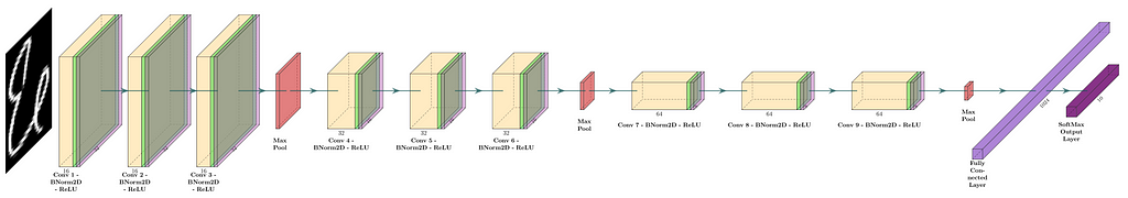
In standard practice, BN2D instances are inserted post-convolution, but pre-activation layers, such as ReLU, as shown in a sample DL network in Figure 1.
Inner Workings of BN2D
An example batch of simple multidimensional spatial data, such as 3-channel images, is shown in Figure 2 to illustrate the internal workings of the BN2D technique.
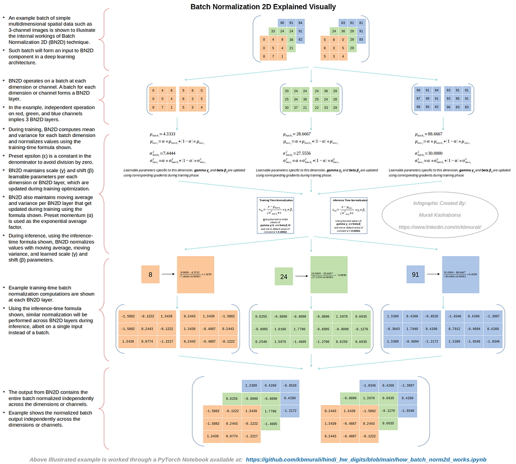
As depicted in Figure 2, BN2D functions by processing a batch at every dimension or channel. If an input batch has N dimensions or channels, the BN2D instance will have N BN2D layers. The separate processing of red, green, and blue channels in the example case implies that the corresponding BN2D instance has 3 BN2D layers.
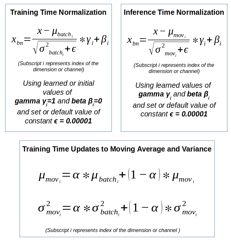
During training, BN2D computes mean and variance for each batch dimension and normalizes values as illustrated in Figure 2 using the training-time formula shown in Figure 3. Preset epsilon (ε) is a constant in the denominator to avoid division by zero. BN2D instance maintains scale (γ) and shift (β) learnable parameters per each dimension or BN2D layer, which are updated during training optimization. BN2D instance also maintains moving average and variance per BN2D layer, as illustrated in Figure 2, which get updated during training using the formula shown in Figure 3. Preset momentum (α) is used as the exponential average factor.
During inference, using the inference-time formula as shown in Figure 3, a BN2D instance normalizes values for each dimension using dimension-specific moving average, moving variance, and learned scale (γ) and shift (β) parameters. Example training-time batch normalization computations are shown in Figure 2 for each dimension in the batch input. The example in Figure 2 also illustrates the output from a BN2D instance containing the entire batch normalized independently across the dimensions or channels. The PyTorch Jupyter Notebook used to work through the example illustrated in Figure 2 is available at the following GitHub repository.
https://github.com/kbmurali/hindi_hw_digits/blob/main/how_batch_norm2d_works.ipynb
BN2D in Action
To inspect the expected performance improvements of incorporating BN2D instances in a DL network architecture, a simple (toy-like) image dataset is used to build relatively simpler DL networks with and without BN2D to predict classes. The following are the crucial DL model performance improvements expected with BN2D:
- Improved Generalization: The normalizations introduced by BN2D are expected to improve the generalization of a DL model. In the example, improved inference-time classification accuracy is expected when BN2D layers are introduced in the network.
- Faster Convergence: Introducing BN2D layers is expected to facilitate faster convergence during training, reducing the number of epochs required to achieve optimal performance. In the example, lowered training losses are expected starting at early epochs after introducing BN2D layers.
- Smoother Gradient Descent: Since BN2D normalizes the dimensional data to a standard scale with a mean of 0 and standard deviation of 1, the possibility of oscillations of gradient descent across the larger-scale dimensions is expected to be minimized, and the gradient descent is expected to progress smoothly.
Example Dataset
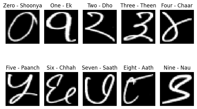
Hindi language hand-written digits (0–9) data published by Kaggle at https://www.kaggle.com/datasets/suvooo/hindi-character-recognition/data (GNU license) is used for training and testing a convolutional DL model with and without BN2D incorporated. Refer to this article’s banner image at the top to see how Hindi digits are written. The DL model network was built using PyTorch DL modules. The choice of hand-written Hindi digits over their English counterparts was based on their complexity compared to the latter. Edge detection in Hindi digits is more challenging than in English due to more curves than straight lines in Hindi digits. Moreover, there could be more variations for the same digit based on one’s writing style.
A utility Python function is developed to make the access to the digits data more PyTorch dataset/dataloader compliant, as shown in the following code snippet. The training dataset had 17000 samples, while the testing dataset had 3000. Note that the PyTorch Grayscale transformer is applied while loading the images as PyTorch Tensors. A utility module, ‘ml_utils.py,’ is specifically developed to package functions for running epochs, training and testing deep learning models using PyTorch Tensor-based operations. The train and test functions also capture model metrics to help evaluate the model’s performance. Python notebooks and utility modules can be accessed at the author’s public GitHub repository, whose link is provided below.
https://github.com/kbmurali/hindi_hw_digits
import torch
import torch.nn as nn
from torch.utils.data import *
import torchvision
from torchvision import transforms
from sklearn.metrics import accuracy_score
import matplotlib.pyplot as plt
import seaborn as sns

from ml_utils import *
from hindi.datasets import Digits

set_seed( 5842 )

batch_size = 32

img_transformer = transforms.Compose([
                        transforms.Grayscale(),
                        transforms.ToTensor()
                    ])

train_dataset = Digits( "./data", train=True, transform=img_transformer, download=True )

test_dataset = Digits( "./data", train=False, transform=img_transformer, download=True )

train_loader = DataLoader( train_dataset, batch_size=batch_size, shuffle=True )

test_loader = DataLoader( test_dataset, batch_size=batch_size )
Example DL Models
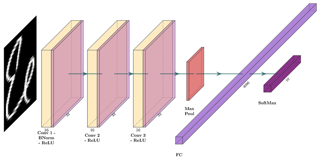
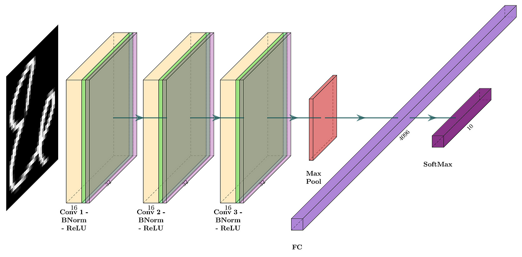
The first DL model will comprise three convolutional layers with 16 filters, each with a kernel size of 3 and padding 1, resulting in the ‘Same’ convolution. The activation function for each convolution is the Rectified Linear Unit (ReLU). The max pooling layer with a pool size 2 is placed before a fully connected layer, leading to a softmax layer producing 10 class outputs. The model’s network architecture is shown in Figure 4. The corresponding PyTorch model definition is shown in the following code snippet.
device = torch.device( 'cuda' if torch.cuda.is_available() else 'cpu' )
loss_func = nn.CrossEntropyLoss()
input_channels = 1
classes = 10
filters = 16
kernel_size = 3
padding = kernel_size//2
pool_size = 2
original_pixels_per_channel = 32*32

three_convs_model = nn.Sequential(
                                    nn.Conv2d( input_channels, filters, kernel_size, padding=padding ), # 1x32x32 => 16x32x32
                                    nn.ReLU(inplace=True), #16x32x32 => 16x32x32
                                    nn.Conv2d(filters, filters, kernel_size, padding=padding ), # 16x32x32 => 16x32x32
                                    nn.ReLU(inplace=True), #16x32x32 => 16x32x32
                                    nn.Conv2d(filters, filters, kernel_size, padding=padding ), # 16x32x32 => 16x32x32
                                    nn.ReLU(inplace=True), #16x32x32 => 16x32x32
                                    nn.MaxPool2d(pool_size), # 16x32x32 => 16x16x16

                                    nn.Flatten(), # 16x16x16 => 4096
                                    nn.Linear( 4096, classes) # 1024 => 10
                                )
The second DL model shares a similar structure to the first one but introduces BN2D instances after convolution and before activation. The model’s network architecture is shown in Figure 5. The corresponding PyTorch model definition is shown in the following code snippet.
three_convs_wth_bn_model = nn.Sequential(
                                            nn.Conv2d( input_channels, filters, kernel_size, padding=padding ), # 1x32x32 => 16x32x32
                                            nn.BatchNorm2d( filters ), #16x32x32 => 16x32x32
                                            nn.ReLU(inplace=True), #16x32x32 => 16x32x32
                                            nn.Conv2d(filters, filters, kernel_size, padding=padding ), # 16x32x32 => 16x32x32
                                            nn.BatchNorm2d( filters ), #16x32x32 => 16x32x32
                                            nn.ReLU(inplace=True), #16x32x32 => 16x32x32
                                            nn.MaxPool2d(pool_size), # 16x32x32 => 16x16x16

                                            nn.Flatten(), # 16x16x16 => 4096
                                            nn.Linear( 4096, classes) # 4096 => 10
                                       )
The two DL models are trained on the example Hindi digits dataset using the utility function shown in the following code snippet. Note that two sample weights from two dimensions/channels of a filter in the last convolutional layer are captured to visualize the training loss’s gradient descent.
three_convs_model_results_df = train_model(
                                            three_convs_model,
                                            loss_func,
                                            train_loader,
                                            test_loader=test_loader,
                                            score_funcs={'accuracy': accuracy_score},
                                            device=device,
                                            epochs=30,
                                            capture_conv_sample_weights=True,
                                            conv_index=4,
                                            wx_flt_index=3,
                                            wx_ch_index=4,
                                            wx_ro_index=1,
                                            wx_index=0,
                                            wy_flt_index=3,
                                            wy_ch_index=8,
                                            wy_ro_index=1,
                                            wy_index=0
                                         )

three_convs_wth_bn_model_results_df = train_model(
                                                    three_convs_wth_bn_model,
                                                    loss_func,
                                                    train_loader,
                                                    test_loader=test_loader,
                                                    score_funcs={'accuracy': accuracy_score},
                                                    device=device,
                                                    epochs=30,
                                                    capture_conv_sample_weights=True,
                                                    conv_index=6,
                                                    wx_flt_index=3,
                                                    wx_ch_index=4,
                                                    wx_ro_index=1,
                                                    wx_index=0,
                                                    wy_flt_index=3,
                                                    wy_ch_index=8,
                                                    wy_ro_index=1,
                                                    wy_index=0
                                                 )
Finding 1: Improved Test Accuracy
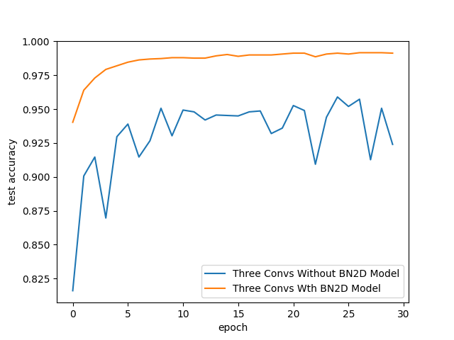
The testing accuracy of the DL model was better with BN2D instances, as shown in Figure 6. The testing accuracy improved gradually with training epochs for the model with BN2D, while it oscillated with training epochs for the model without BN2D. At the end of epoch 30, the test accuracy for the model with BN2D was 99.1%, while 92.4% for the model without BN2D. These results suggest that incorporating BN2D instances positively affected the model’s performance, significantly increasing the testing accuracy.
sns.lineplot( x='epoch', y='test accuracy', data=three_convs_model_results_df, label="Three Convs Without BN2D Model" )
sns.lineplot( x='epoch', y='test accuracy', data=three_convs_wth_bn_model_results_df, label="Three Convs Wth BN2D Model" )
Finding 2: Faster Convergence
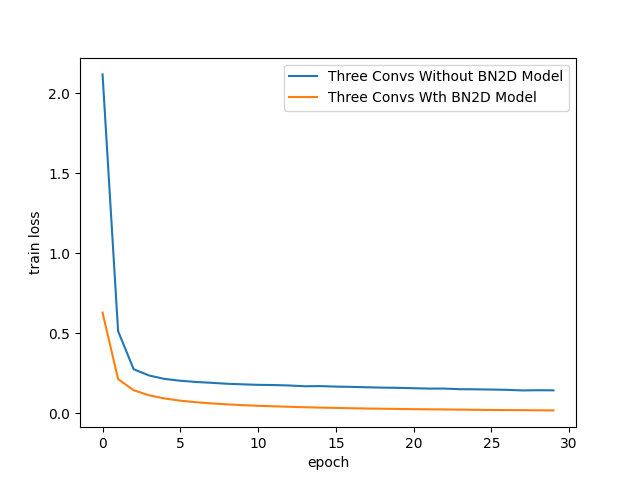
The training loss of the DL model was much lower with BN2D instances, as shown in Figure 7. By around training epoch 3 itself, the model with BN2D manifested lower training losses than without BN2D. The lower training losses suggest that BN2D facilitates faster convergence during training, perhaps reducing the number of training epochs for reasonable convergence.
sns.lineplot( x='epoch', y='train loss', data=three_convs_model_results_df, label="Three Convs Without BN2D Model" )
sns.lineplot( x='epoch', y='train loss', data=three_convs_wth_bn_model_results_df, label="Three Convs Wth BN2D Model" )
Finding 3: Smoother Gradient Descent
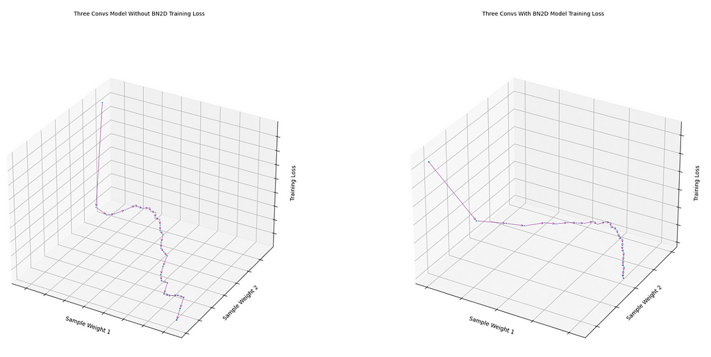
The loss function over the two sample weights taken from the last convolution of the model with BN2D manifested smoother gradient descent than without BN2D, as shown in Figure 8. The loss function of the model without BN2D followed a rather zig-zag gradient descent. The smoother gradient descent with BN2D suggests that normalizing the dimensional data to a standard scale with a mean of 0 and standard deviation of 1 enables weights of different dimensions possibly to be on a similar scale, reducing the possible oscillations of the gradient descent.
fig1 = draw_loss_descent( three_convs_model_results_df, title='Three Convs Model Without BN2D Training Loss' )
fig2 = draw_loss_descent( three_convs_wth_bn_model_results_df, title='Three Convs With BN2D Model Training Loss' )
Practical Considerations
While the benefits of BN2D are clear, its implementation requires careful consideration. Proper initialization of weights, suitable learning rates, and the placement of BN2D layers within the DL network are crucial factors to maximize its effectiveness. While BN2D often prevents over-fitting, there can be cases where it may even contribute to over-fitting under certain circumstances. For example, if BN2D is used along with another technique called Dropout, the combination might have different effects on over-fitting depending on the specific configuration and the dataset. Likewise, in the case of small batch sizes, the batch mean and variance may not closely represent the overall dataset statistics, potentially resulting in noisy normalization, which may not be as effective in preventing over-fitting.
Conclusion
The write-up intended to showcase the intuitions behind using BN2D in deep learning networks. The example convolutional models using toy-like image data were solely to showcase expected performance improvements incorporating BN2D instances in a DL network architecture. The BN2D normalization across spatial and channel dimensions brings about training stability, faster convergence, and enhanced generalization, ultimately contributing to the success of deep learning models. Hopefully, the write-up gives a good understanding of how BN2D works and the intuition behind it. Such understanding and intuition come in handy while developing more complex DL models.
References:
- Hindi Character Recognition
- BatchNorm2d – PyTorch 2.1 documentation
- Why 2D batch normalisation is used in features and 1D in classifiers?
- Keras documentation: BatchNormalization layer
Exploring the Superhero Role of 2D Batch Normalization in Deep Learning Architectures was originally published in Towards Data Science on Medium, where people are continuing the conversation by highlighting and responding to this story.
Internal working and intuitions are explained through simple examples
Deep Learning (DL) has been a game-changer in the evolution of Convolutional Neural Networks (CNN) and Generative Artificial Intelligence (Gen AI). Such DL models can extract complex patterns and features from multidimensional spatial data, such as images, and make predictions. The more intricate the patterns in the input data are, the more complex can the model architecture be. There are many ways to accelerate the model training convergence and enhance the model inference performance, but Batch Normalization 2D (BN2D) has emerged as a superhero in this area. This write-up aims to showcase how integrating BN2D in a DL architecture can lead to faster convergence and better inference.
Understanding BN2D
BN2D is a normalization technique applied in batches to multidimensional spatial inputs such as images to normalize their dimensional (channel) values so that dimensions across such batches have a mean of 0 and a variance of 1.
The primary purpose of incorporating BN2D components is to prevent internal covariate shifts across dimensions or channels in input data from previous layers within a network. Internal covariate shifts across dimensions occur when the distributions of dimensional data change due to updates made to network parameters during training epochs. For instance, N filters in a convolutional layer produce N-dimensional activations as output. This layer maintains weight and bias parameters for its filters that get updated incrementally with each training epoch.
As a result of these updates, activations from one filter can have a markedly different distribution than activations from another of the same convolutional layer. Such differences in distribution indicate that activations from one filter are on a vastly different scale than activations from another filter. When inputting such dimensional data with vastly different scales to the next layer in the network, the learnability of that layer is hindered because the weights of dimensions with larger scales require larger updates during gradient descent than those with smaller scales.
The other possible consequence is that gradients of weights with smaller scales can vanish, while gradients of weights with larger scales can explode. When the network experiences such learning obstacles, gradient descent will oscillate across the larger-scale dimensions, severely hindering learning convergence and training stability. BN2D effectively mitigates this phenomenon by normalizing the dimensional data to a standard scale with a mean of 0 and standard deviation of 1 and facilitates faster convergence during training, reducing the number of epochs required to achieve optimal performance. As such, by easing the network’s training phase, the technique ensures that the network can focus on learning more complex and abstract features, allowing the extraction of richer representations from the input data.
In standard practice, BN2D instances are inserted post-convolution, but pre-activation layers, such as ReLU, as shown in a sample DL network in Figure 1.
Inner Workings of BN2D
An example batch of simple multidimensional spatial data, such as 3-channel images, is shown in Figure 2 to illustrate the internal workings of the BN2D technique.
As depicted in Figure 2, BN2D functions by processing a batch at every dimension or channel. If an input batch has N dimensions or channels, the BN2D instance will have N BN2D layers. The separate processing of red, green, and blue channels in the example case implies that the corresponding BN2D instance has 3 BN2D layers.
During training, BN2D computes mean and variance for each batch dimension and normalizes values as illustrated in Figure 2 using the training-time formula shown in Figure 3. Preset epsilon (ε) is a constant in the denominator to avoid division by zero. BN2D instance maintains scale (γ) and shift (β) learnable parameters per each dimension or BN2D layer, which are updated during training optimization. BN2D instance also maintains moving average and variance per BN2D layer, as illustrated in Figure 2, which get updated during training using the formula shown in Figure 3. Preset momentum (α) is used as the exponential average factor.
During inference, using the inference-time formula as shown in Figure 3, a BN2D instance normalizes values for each dimension using dimension-specific moving average, moving variance, and learned scale (γ) and shift (β) parameters. Example training-time batch normalization computations are shown in Figure 2 for each dimension in the batch input. The example in Figure 2 also illustrates the output from a BN2D instance containing the entire batch normalized independently across the dimensions or channels. The PyTorch Jupyter Notebook used to work through the example illustrated in Figure 2 is available at the following GitHub repository.
https://github.com/kbmurali/hindi_hw_digits/blob/main/how_batch_norm2d_works.ipynb
BN2D in Action
To inspect the expected performance improvements of incorporating BN2D instances in a DL network architecture, a simple (toy-like) image dataset is used to build relatively simpler DL networks with and without BN2D to predict classes. The following are the crucial DL model performance improvements expected with BN2D:
- Improved Generalization: The normalizations introduced by BN2D are expected to improve the generalization of a DL model. In the example, improved inference-time classification accuracy is expected when BN2D layers are introduced in the network.
- Faster Convergence: Introducing BN2D layers is expected to facilitate faster convergence during training, reducing the number of epochs required to achieve optimal performance. In the example, lowered training losses are expected starting at early epochs after introducing BN2D layers.
- Smoother Gradient Descent: Since BN2D normalizes the dimensional data to a standard scale with a mean of 0 and standard deviation of 1, the possibility of oscillations of gradient descent across the larger-scale dimensions is expected to be minimized, and the gradient descent is expected to progress smoothly.
Example Dataset
Hindi language hand-written digits (0–9) data published by Kaggle at https://www.kaggle.com/datasets/suvooo/hindi-character-recognition/data (GNU license) is used for training and testing a convolutional DL model with and without BN2D incorporated. Refer to this article’s banner image at the top to see how Hindi digits are written. The DL model network was built using PyTorch DL modules. The choice of hand-written Hindi digits over their English counterparts was based on their complexity compared to the latter. Edge detection in Hindi digits is more challenging than in English due to more curves than straight lines in Hindi digits. Moreover, there could be more variations for the same digit based on one’s writing style.
A utility Python function is developed to make the access to the digits data more PyTorch dataset/dataloader compliant, as shown in the following code snippet. The training dataset had 17000 samples, while the testing dataset had 3000. Note that the PyTorch Grayscale transformer is applied while loading the images as PyTorch Tensors. A utility module, ‘ml_utils.py,’ is specifically developed to package functions for running epochs, training and testing deep learning models using PyTorch Tensor-based operations. The train and test functions also capture model metrics to help evaluate the model’s performance. Python notebooks and utility modules can be accessed at the author’s public GitHub repository, whose link is provided below.
https://github.com/kbmurali/hindi_hw_digits
import torch
import torch.nn as nn
from torch.utils.data import *
import torchvision
from torchvision import transforms
from sklearn.metrics import accuracy_score
import matplotlib.pyplot as plt
import seaborn as sns

from ml_utils import *
from hindi.datasets import Digits

set_seed( 5842 )

batch_size = 32

img_transformer = transforms.Compose([
                        transforms.Grayscale(),
                        transforms.ToTensor()
                    ])

train_dataset = Digits( "./data", train=True, transform=img_transformer, download=True )

test_dataset = Digits( "./data", train=False, transform=img_transformer, download=True )

train_loader = DataLoader( train_dataset, batch_size=batch_size, shuffle=True )

test_loader = DataLoader( test_dataset, batch_size=batch_size )
Example DL Models
The first DL model will comprise three convolutional layers with 16 filters, each with a kernel size of 3 and padding 1, resulting in the ‘Same’ convolution. The activation function for each convolution is the Rectified Linear Unit (ReLU). The max pooling layer with a pool size 2 is placed before a fully connected layer, leading to a softmax layer producing 10 class outputs. The model’s network architecture is shown in Figure 4. The corresponding PyTorch model definition is shown in the following code snippet.
device = torch.device( 'cuda' if torch.cuda.is_available() else 'cpu' )
loss_func = nn.CrossEntropyLoss()
input_channels = 1
classes = 10
filters = 16
kernel_size = 3
padding = kernel_size//2
pool_size = 2
original_pixels_per_channel = 32*32

three_convs_model = nn.Sequential(
                                    nn.Conv2d( input_channels, filters, kernel_size, padding=padding ), # 1x32x32 => 16x32x32
                                    nn.ReLU(inplace=True), #16x32x32 => 16x32x32
                                    nn.Conv2d(filters, filters, kernel_size, padding=padding ), # 16x32x32 => 16x32x32
                                    nn.ReLU(inplace=True), #16x32x32 => 16x32x32
                                    nn.Conv2d(filters, filters, kernel_size, padding=padding ), # 16x32x32 => 16x32x32
                                    nn.ReLU(inplace=True), #16x32x32 => 16x32x32
                                    nn.MaxPool2d(pool_size), # 16x32x32 => 16x16x16

                                    nn.Flatten(), # 16x16x16 => 4096
                                    nn.Linear( 4096, classes) # 1024 => 10
                                )
The second DL model shares a similar structure to the first one but introduces BN2D instances after convolution and before activation. The model’s network architecture is shown in Figure 5. The corresponding PyTorch model definition is shown in the following code snippet.
three_convs_wth_bn_model = nn.Sequential(
                                            nn.Conv2d( input_channels, filters, kernel_size, padding=padding ), # 1x32x32 => 16x32x32
                                            nn.BatchNorm2d( filters ), #16x32x32 => 16x32x32
                                            nn.ReLU(inplace=True), #16x32x32 => 16x32x32
                                            nn.Conv2d(filters, filters, kernel_size, padding=padding ), # 16x32x32 => 16x32x32
                                            nn.BatchNorm2d( filters ), #16x32x32 => 16x32x32
                                            nn.ReLU(inplace=True), #16x32x32 => 16x32x32
                                            nn.Conv2d(filters, filters, kernel_size, padding=padding ), # 16x32x32 => 16x32x32
                                            nn.BatchNorm2d( filters ), #16x32x32 => 16x32x32
                                            nn.ReLU(inplace=True), #16x32x32 => 16x32x32
                                            nn.MaxPool2d(pool_size), # 16x32x32 => 16x16x16

                                            nn.Flatten(), # 16x16x16 => 4096
                                            nn.Linear( 4096, classes) # 4096 => 10
                                       )
The two DL models are trained on the example Hindi digits dataset using the utility function shown in the following code snippet. Note that two sample weights from two dimensions/channels of a filter in the last convolutional layer are captured to visualize the training loss’s gradient descent.
three_convs_model_results_df = train_model(
                                            three_convs_model,
                                            loss_func,
                                            train_loader,
                                            test_loader=test_loader,
                                            score_funcs={'accuracy': accuracy_score},
                                            device=device,
                                            epochs=30,
                                            capture_conv_sample_weights=True,
                                            conv_index=4,
                                            wx_flt_index=3,
                                            wx_ch_index=4,
                                            wx_ro_index=1,
                                            wx_index=0,
                                            wy_flt_index=3,
                                            wy_ch_index=8,
                                            wy_ro_index=1,
                                            wy_index=0
                                         )

three_convs_wth_bn_model_results_df = train_model(
                                                    three_convs_wth_bn_model,
                                                    loss_func,
                                                    train_loader,
                                                    test_loader=test_loader,
                                                    score_funcs={'accuracy': accuracy_score},
                                                    device=device,
                                                    epochs=30,
                                                    capture_conv_sample_weights=True,
                                                    conv_index=6,
                                                    wx_flt_index=3,
                                                    wx_ch_index=4,
                                                    wx_ro_index=1,
                                                    wx_index=0,
                                                    wy_flt_index=3,
                                                    wy_ch_index=8,
                                                    wy_ro_index=1,
                                                    wy_index=0
                                                 )
Finding 1: Improved Test Accuracy
The testing accuracy of the DL model was better with BN2D instances, as shown in Figure 6. The testing accuracy improved gradually with training epochs for the model with BN2D, while it oscillated with training epochs for the model without BN2D. At the end of epoch 30, the test accuracy for the model with BN2D was 99.1%, while 92.4% for the model without BN2D. These results suggest that incorporating BN2D instances positively affected the model’s performance, significantly increasing the testing accuracy.
sns.lineplot( x='epoch', y='test accuracy', data=three_convs_model_results_df, label="Three Convs Without BN2D Model" )
sns.lineplot( x='epoch', y='test accuracy', data=three_convs_wth_bn_model_results_df, label="Three Convs Wth BN2D Model" )
Finding 2: Faster Convergence
The training loss of the DL model was much lower with BN2D instances, as shown in Figure 7. By around training epoch 3 itself, the model with BN2D manifested lower training losses than without BN2D. The lower training losses suggest that BN2D facilitates faster convergence during training, perhaps reducing the number of training epochs for reasonable convergence.
sns.lineplot( x='epoch', y='train loss', data=three_convs_model_results_df, label="Three Convs Without BN2D Model" )
sns.lineplot( x='epoch', y='train loss', data=three_convs_wth_bn_model_results_df, label="Three Convs Wth BN2D Model" )
Finding 3: Smoother Gradient Descent
The loss function over the two sample weights taken from the last convolution of the model with BN2D manifested smoother gradient descent than without BN2D, as shown in Figure 8. The loss function of the model without BN2D followed a rather zig-zag gradient descent. The smoother gradient descent with BN2D suggests that normalizing the dimensional data to a standard scale with a mean of 0 and standard deviation of 1 enables weights of different dimensions possibly to be on a similar scale, reducing the possible oscillations of the gradient descent.
fig1 = draw_loss_descent( three_convs_model_results_df, title='Three Convs Model Without BN2D Training Loss' )
fig2 = draw_loss_descent( three_convs_wth_bn_model_results_df, title='Three Convs With BN2D Model Training Loss' )
Practical Considerations
While the benefits of BN2D are clear, its implementation requires careful consideration. Proper initialization of weights, suitable learning rates, and the placement of BN2D layers within the DL network are crucial factors to maximize its effectiveness. While BN2D often prevents over-fitting, there can be cases where it may even contribute to over-fitting under certain circumstances. For example, if BN2D is used along with another technique called Dropout, the combination might have different effects on over-fitting depending on the specific configuration and the dataset. Likewise, in the case of small batch sizes, the batch mean and variance may not closely represent the overall dataset statistics, potentially resulting in noisy normalization, which may not be as effective in preventing over-fitting.
Conclusion
The write-up intended to showcase the intuitions behind using BN2D in deep learning networks. The example convolutional models using toy-like image data were solely to showcase expected performance improvements incorporating BN2D instances in a DL network architecture. The BN2D normalization across spatial and channel dimensions brings about training stability, faster convergence, and enhanced generalization, ultimately contributing to the success of deep learning models. Hopefully, the write-up gives a good understanding of how BN2D works and the intuition behind it. Such understanding and intuition come in handy while developing more complex DL models.
References:
- Hindi Character Recognition
- BatchNorm2d – PyTorch 2.1 documentation
- Why 2D batch normalisation is used in features and 1D in classifiers?
- Keras documentation: BatchNormalization layer
Exploring the Superhero Role of 2D Batch Normalization in Deep Learning Architectures was originally published in Towards Data Science on Medium, where people are continuing the conversation by highlighting and responding to this story.
Denial of responsibility! Techno Blender is an automatic aggregator of the all world’s media. In each content, the hyperlink to the primary source is specified. All trademarks belong to their rightful owners, all materials to their authors. If you are the owner of the content and do not want us to publish your materials, please contact us by email – [email protected]. The content will be deleted within 24 hours.