
Exposing the Power of the Kalman Filter
As a data scientist we are occasionally faced with situations where we need to model a trend to predict future values. Whilst there is a temptation to focus on statistical or machine learning based algorithms, I am here to present a different option: the Kalman Filter (KF).
In the early 1960’s Rudolf E. Kalman revolutionised how complex systems can be modelled with the KF. From guiding aircrafts or spacecrafts to their destination to allowing you smartphone to find its place in this world, this algorithm blends data and mathematics to provide estimates of future states with incredible accuracy.
In this blog we will go in-depth to cover how the Kalman Filter works, showing examples in Python that will emphasise the true power of this technique. Starting with a simple 2D example, we will see how we can modify the code to adapt it to more advanced 4D spaces and end by covering the Extended Kalman Filter (the sophisticated predecessor). Join me on this journey as we embark through the world of predictive algorithms and filters.
The basics of a Kalman filter
The KF provides an estimate of the state of a system by building and continuously updating a set of covariance matrices (representing the statistical distribution of noise and past states) collected from observations and other measurements in time. Unlike other out-of-the-box algorithms, it is possible to directly expand and refine the solution by defining the mathematical relationships between the system and external sources. Whilst this might sound quite complex and intricate, the process can be summarised down to two steps: predict and update. These phases work together to iteratively correct and refine the state estimates of the system.
Predict step:
This phase is all about forecasting the next future state of the system based on the model’s known posteriori estimates and step in time of Δk. Mathematically we represent the estimates of the state space as:

where, F, our state transition matrix models how the states evolve one step to another irrespective of the control input and process noise. Our matrix B models the control input, uₖ, impact on the state.
Alongside our estimates of the next state, the algorithm also calculates the uncertainty of the estimate represented by the covariance matrix P:
The predicted state covariance matrix represents the confidence and accuracy of our predictions, influenced by Q the process noise covariance matrix from the system itself. We apply this matrix to subsiquent equations in the update step to correct the information the Kalman Filter holds on the system, subsiquently improving future state estimates.
Update step:
In the update step the algorithm performs updates to the Kalman Gain, State estimates and the Covariance matrix. The Kalman Gain determines how much influence a new measurement should have on the state estimates. The calculation includes the observation model matrix, H, which relates the state to the measurement we expect to receive, and R the measurement noise covariance matrix of errors in the measurments:

In essence, K attempts to balance uncertainty in the predictions with that present in the measurements. As mentioned above, the Kalman Gain is applied to correct the state estimates and covariance, as presented by the following equations respectively:

where the calculation in the brackets for the state estimate is the residual, the difference between the actual measurement and that which the model predicted.
The true beauty of how a Kalman Filter works lies in its recursive nature, continuously updating both the state and covariance as new information is received. This allows the model to refine in a statistically optimal way over time which is particularly powerful approach to modelling systems that receive a stream of noisy observations.
The Kalman filter in action
It is possible to become quite overwhelmed by the equations that underpin the Kalman Filter, and to fully appreciate how it works from the mathematics alone would require an understanding of state space (out of the scope of this blog), but I will try to bring it to life with some Python examples. In it’s simplest form, we can define a Kalman Filter object as:
import numpy as np

class KalmanFilter:
    """
    An implementation of the classic Kalman Filter for linear dynamic systems.
    The Kalman Filter is an optimal recursive data processing algorithm which
    aims to estimate the state of a system from noisy observations.

    Attributes:
        F (np.ndarray): The state transition matrix.
        B (np.ndarray): The control input marix.
        H (np.ndarray): The observation matrix.
        u (np.ndarray): the control input.
        Q (np.ndarray): The process noise covariance matrix.
        R (np.ndarray): The measurement noise covariance matrix.
        x (np.ndarray): The mean state estimate of the previous step (k-1).
        P (np.ndarray): The state covariance of previous step (k-1).
    """
    def __init__(self, F, B, u, H, Q, R, x0, P0):
        """
        Initializes the Kalman Filter with the necessary matrices and initial state.

        Parameters:
            F (np.ndarray): The state transition matrix.
            B (np.ndarray): The control input marix.
            H (np.ndarray): The observation matrix.
            u (np.ndarray): the control input.
            Q (np.ndarray): The process noise covariance matrix.
            R (np.ndarray): The measurement noise covariance matrix.
            x0 (np.ndarray): The initial state estimate.
            P0 (np.ndarray): The initial state covariance matrix.
        """
        self.F = F  # State transition matrix
        self.B = B  # Control input matrix
        self.u = u  # Control vector
        self.H = H  # Observation matrix
        self.Q = Q  # Process noise covariance
        self.R = R  # Measurement noise covariance
        self.x = x0  # Initial state estimate
        self.P = P0  # Initial estimate covariance

    def predict(self):
        """
        Predicts the state and the state covariance for the next time step.
        """
        self.x = self.F @ self.x + self.B @ self.u
        self.P = self.F @ self.P @ self.F.T + self.Q
        return self.x

    def update(self, z):
        """
        Updates the state estimate with the latest measurement.

        Parameters:
            z (np.ndarray): The measurement at the current step.
        """
        y = z - self.H @ self.x
        S = self.H @ self.P @ self.H.T + self.R
        K = self.P @ self.H.T @ np.linalg.inv(S)
        self.x = self.x + K @ y
        I = np.eye(self.P.shape[0])
        self.P = (I - K @ self.H) @ self.P

        return self.xChallenges with Non-linear Systems
We will use the predict() and update() functions to iterate through the steps outlined earlier. The above design of the filter will work for any time-series, and to show how our estimates compare to actuals let’s construct a simple example:
import numpy as np
import matplotlib.pyplot as plt

# Set the random seed for reproducibility
np.random.seed(42)

# Simulate the ground truth position of the object
true_velocity = 0.5  # units per time step
num_steps = 50
time_steps = np.linspace(0, num_steps, num_steps)
true_positions = true_velocity * time_steps

# Simulate the measurements with noise
measurement_noise = 10  # increase this value to make measurements noisier
noisy_measurements = true_positions + np.random.normal(0, measurement_noise, num_steps)

# Plot the true positions and the noisy measurements
plt.figure(figsize=(10, 6))
plt.plot(time_steps, true_positions, label='True Position', color='green')
plt.scatter(time_steps, noisy_measurements, label='Noisy Measurements', color='red', marker='o')

plt.xlabel('Time Step')
plt.ylabel('Position')
plt.title('True Position and Noisy Measurements Over Time')
plt.legend()
plt.show()
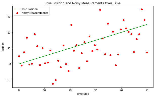
In reality the ‘True Position’ would be unknown but we will plot it here for reference, the ‘Noisy Measurements’ are the observation points that are fed into our Kalman Filter. We will perform a very basic instantiation of the matrices, and to some degree it does not matter as the Kalman model will converge quickly through application of the Kalman Gain, but it might be reasonable under certain circumstances to perform a warm start to the model.
# Kalman Filter Initialization
F = np.array([[1, 1], [0, 1]])   # State transition matrix
B = np.array([[0], [0]])          # No control input
u = np.array([[0]])               # No control input
H = np.array([[1, 0]])            # Measurement function
Q = np.array([[1, 0], [0, 3]])    # Process noise covariance
R = np.array([[measurement_noise**2]]) # Measurement noise covariance
x0 = np.array([[0], [0]])         # Initial state estimate
P0 = np.array([[1, 0], [0, 1]])   # Initial estimate covariance

kf = KalmanFilter(F, B, u, H, Q, R, x0, P0)

# Allocate space for estimated positions and velocities
estimated_positions = np.zeros(num_steps)
estimated_velocities = np.zeros(num_steps)

# Kalman Filter Loop
for t in range(num_steps):
    # Predict
    kf.predict()

    # Update
    measurement = np.array([[noisy_measurements[t]]])
    kf.update(measurement)

    # Store the filtered position and velocity
    estimated_positions[t] = kf.x[0]
    estimated_velocities[t] = kf.x[1]

# Plot the true positions, noisy measurements, and the Kalman filter estimates
plt.figure(figsize=(10, 6))
plt.plot(time_steps, true_positions, label='True Position', color='green')
plt.scatter(time_steps, noisy_measurements, label='Noisy Measurements', color='red', marker='o')
plt.plot(time_steps, estimated_positions, label='Kalman Filter Estimate', color='blue')

plt.xlabel('Time Step')
plt.ylabel('Position')
plt.title('Kalman Filter Estimation Over Time')
plt.legend()
plt.show()

Even with this very simple design of a solution, the model does an okay job piercing through the noise to find the true position. This might work okay for simple applications but often trends are more nuanced and impacted by external events. To handle this we typically need to modify both the state space representation but also the way we calculate estimates and correct the covariance matrix when new information arrives, let’s explore this more with another example
Tracking a moving object in 4D
Let’s assume we want to track the movement of an object in space and time, and to make this example even more realistic we will simulate some force acting upon it resulting in angular rotation. To show the adaptability of this algorithm to higher dimensional state space representations we will assume a linear force, although in actuality this will not be the case (we will explore a more realistic example after this). The below code shows an example of how we would modify our Kalman Filter for this particular scenario.
import numpy as np
import matplotlib.pyplot as plt
from mpl_toolkits.mplot3d import Axes3D

class KalmanFilter:
    """
    An implementation of the classic Kalman Filter for linear dynamic systems.
    The Kalman Filter is an optimal recursive data processing algorithm which
    aims to estimate the state of a system from noisy observations.

    Attributes:
        F (np.ndarray): The state transition matrix.
        B (np.ndarray): The control input marix.
        H (np.ndarray): The observation matrix.
        u (np.ndarray): the control input.
        Q (np.ndarray): The process noise covariance matrix.
        R (np.ndarray): The measurement noise covariance matrix.
        x (np.ndarray): The mean state estimate of the previous step (k-1).
        P (np.ndarray): The state covariance of previous step (k-1).
    """
    def __init__(self, F=None, B=None, u=None, H=None, Q=None, R=None, x0=None, P0=None):
        """
        Initializes the Kalman Filter with the necessary matrices and initial state.

        Parameters:
            F (np.ndarray): The state transition matrix.
            B (np.ndarray): The control input marix.
            H (np.ndarray): The observation matrix.
            u (np.ndarray): the control input.
            Q (np.ndarray): The process noise covariance matrix.
            R (np.ndarray): The measurement noise covariance matrix.
            x0 (np.ndarray): The initial state estimate.
            P0 (np.ndarray): The initial state covariance matrix.
        """
        self.F = F  # State transition matrix
        self.B = B  # Control input matrix
        self.u = u  # Control input
        self.H = H  # Observation matrix
        self.Q = Q  # Process noise covariance
        self.R = R  # Measurement noise covariance
        self.x = x0  # Initial state estimate
        self.P = P0  # Initial estimate covariance

    def predict(self):
        """
        Predicts the state and the state covariance for the next time step.
        """
        self.x = np.dot(self.F, self.x) + np.dot(self.B, self.u)
        self.P = np.dot(np.dot(self.F, self.P), self.F.T) + self.Q

    def update(self, z):
        """
        Updates the state estimate with the latest measurement.

        Parameters:
            z (np.ndarray): The measurement at the current step.
        """
        y = z - np.dot(self.H, self.x)
        S = np.dot(self.H, np.dot(self.P, self.H.T)) + self.R
        K = np.dot(np.dot(self.P, self.H.T), np.linalg.inv(S))
        self.x = self.x + np.dot(K, y)
        self.P = self.P - np.dot(np.dot(K, self.H), self.P)

# Parameters for simulation
true_angular_velocity = 0.1  # radians per time step
radius = 20
num_steps = 100
dt = 1  # time step

# Create time steps
time_steps = np.arange(0, num_steps*dt, dt)

# Ground truth state
true_x_positions = radius * np.cos(true_angular_velocity * time_steps)
true_y_positions = radius * np.sin(true_angular_velocity * time_steps)
true_z_positions = 0.5 * time_steps  # constant velocity in z

# Create noisy measurements
measurement_noise = 1.0
noisy_x_measurements = true_x_positions + np.random.normal(0, measurement_noise, num_steps)
noisy_y_measurements = true_y_positions + np.random.normal(0, measurement_noise, num_steps)
noisy_z_measurements = true_z_positions + np.random.normal(0, measurement_noise, num_steps)

# Kalman Filter initialization
F = np.array([[1, 0, 0, -radius*dt*np.sin(true_angular_velocity*dt)],
              [0, 1, 0, radius*dt*np.cos(true_angular_velocity*dt)],
              [0, 0, 1, 0],
              [0, 0, 0, 1]])
B = np.zeros((4, 1))
u = np.zeros((1, 1))
H = np.array([[1, 0, 0, 0],
              [0, 1, 0, 0],
              [0, 0, 1, 0]])
Q = np.eye(4) * 0.1  # Small process noise
R = measurement_noise**2 * np.eye(3)  # Measurement noise
x0 = np.array([[0], [radius], [0], [true_angular_velocity]])
P0 = np.eye(4) * 1.0

kf = KalmanFilter(F, B, u, H, Q, R, x0, P0)

# Allocate space for estimated states
estimated_states = np.zeros((num_steps, 4))

# Kalman Filter Loop
for t in range(num_steps):
    # Predict
    kf.predict()

    # Update
    z = np.array([[noisy_x_measurements[t]],
                  [noisy_y_measurements[t]],
                  [noisy_z_measurements[t]]])
    kf.update(z)

    # Store the state
    estimated_states[t, :] = kf.x.ravel()

# Extract estimated positions
estimated_x_positions = estimated_states[:, 0]
estimated_y_positions = estimated_states[:, 1]
estimated_z_positions = estimated_states[:, 2]

# Plotting
fig = plt.figure(figsize=(10, 8))
ax = fig.add_subplot(111, projection='3d')

# Plot the true trajectory
ax.plot(true_x_positions, true_y_positions, true_z_positions, label='True Trajectory', color='g')
# Plot the start and end markers for the true trajectory
ax.scatter(true_x_positions[0], true_y_positions[0], true_z_positions[0], label='Start (Actual)', c='green', marker='x', s=100)
ax.scatter(true_x_positions[-1], true_y_positions[-1], true_z_positions[-1], label='End (Actual)', c='red', marker='x', s=100)


# Plot the noisy measurements
ax.scatter(noisy_x_measurements, noisy_y_measurements, noisy_z_measurements, label='Noisy Measurements', color='r')

# Plot the estimated trajectory
ax.plot(estimated_x_positions, estimated_y_positions, estimated_z_positions, label='Estimated Trajectory', color='b')

# Plot settings
ax.set_xlabel('X position')
ax.set_ylabel('Y position')
ax.set_zlabel('Z position')
ax.set_title('3D Trajectory Estimation with Kalman Filter')
ax.legend()

plt.show()
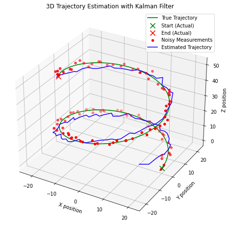
A few interesting point to note here, in the graph above we can see how the model quickly corrects to the estimated true state as we start iterating over the observations. The model also performs reasonably well at identifying the true state of the system, with estimations intersecting with the true states (‘true trajectory’). This design might be appropriate for some real world applications but not for those where the force acting upon the system is nonlinear. Instead we need to consider a different application of the Kalman Filter: the Extended Kalman Filter, a predecessor to what we have explored until now that linearises nonlinearity of the incoming observations.
The Extended Kalman Filter
When attempting to model a system where either the observations or dynamics of the system are nonlinear we need to apply the Extended Kalman Filter (EKF). This algorithm differs to the last by incorporating the Jacobian matrix into the solution and performing Taylor series expansion to find first-order linear approximations of the state transition and observation models. To express this extension mathematically, our key algorithmic calculations now become:
for the state prediction, where f is our nonlinear state transition function applied to the previous state estimate and u the control input at the previous time step.

for the error covariance prediction, where F is the Jacobian of the state transition function with respect to P the previous error covariance and Q the process noise covariance matrix.

the observation of our measurement, z, at time step k, where h is the nonlinear observation function applied to our state prediction with some additive observation noise v.

our update to the Kalman Gain calculation, with H the Jacobian of the observation function with respect to the state and R the measurement noise covariance matrix.

the modified calculation for the state estimate that incorporates the kalman gain and the nonlinear observation function, and finally our equation to update the error covariance:

In the last example this will use the Jocabian to linearise the non-linear affect of angular rotation on our object, modifying the code appropriately. Designing an EKF is more challenged than the KF as we our assumption of first-order linear approximations may inadvertently introduce errors into our state estimates. In addition, the Jacobian calculation can become complex, computationally expensive and difficult to define for certain situations which may also lead to errors. However, if designed correctly, the EKF will often outperform the KF implementation.
Building on our last Python example I have presented the implementation of the EKF:
import numpy as np
import matplotlib.pyplot as plt
from mpl_toolkits.mplot3d import Axes3D

class ExtendedKalmanFilter:
    """
    An implementation of the Extended Kalman Filter (EKF).
    This filter is suitable for systems with non-linear dynamics by linearising
    the system model at each time step using the Jacobian.

    Attributes:
        state_transition (callable): The state transition function for the system.
        jacobian_F (callable): Function to compute the Jacobian of the state transition.
        H (np.ndarray): The observation matrix.
        jacobian_H (callable): Function to compute the Jacobian of the observation model.
        Q (np.ndarray): The process noise covariance matrix.
        R (np.ndarray): The measurement noise covariance matrix.
        x (np.ndarray): The initial state estimate.
        P (np.ndarray): The initial estimate covariance.
    """
    def __init__(self, state_transition, jacobian_F, observation_matrix, jacobian_H, Q, R, x, P):
        """
        Constructs the Extended Kalman Filter.

        Parameters:
            state_transition (callable): The state transition function.
            jacobian_F (callable): Function to compute the Jacobian of F.
            observation_matrix (np.ndarray): Observation matrix.
            jacobian_H (callable): Function to compute the Jacobian of H.
            Q (np.ndarray): Process noise covariance.
            R (np.ndarray): Measurement noise covariance.
            x (np.ndarray): Initial state estimate.
            P (np.ndarray): Initial estimate covariance.
        """
        self.state_transition = state_transition  # Non-linear state transition function
        self.jacobian_F = jacobian_F  # Function to compute Jacobian of F
        self.H = observation_matrix  # Observation matrix
        self.jacobian_H = jacobian_H  # Function to compute Jacobian of H
        self.Q = Q  # Process noise covariance
        self.R = R  # Measurement noise covariance
        self.x = x  # Initial state estimate
        self.P = P  # Initial estimate covariance

    def predict(self, u):
        """
        Predicts the state at the next time step.

        Parameters:
            u (np.ndarray): The control input vector.
        """
        self.x = self.state_transition(self.x, u)
        F = self.jacobian_F(self.x, u)
        self.P = F @ self.P @ F.T + self.Q

    def update(self, z):
        """
        Updates the state estimate with a new measurement.

        Parameters:
            z (np.ndarray): The measurement vector.
        """
        H = self.jacobian_H()
        y = z - self.H @ self.x
        S = H @ self.P @ H.T + self.R
        K = self.P @ H.T @ np.linalg.inv(S)
        self.x = self.x + K @ y
        self.P = (np.eye(len(self.x)) - K @ H) @ self.P

# Define the non-linear transition and Jacobian functions
def state_transition(x, u):
    """
    Defines the state transition function for the system with non-linear dynamics.

    Parameters:
        x (np.ndarray): The current state vector.
        u (np.ndarray): The control input vector containing time step and rate of change of angular velocity.

    Returns:
        np.ndarray: The next state vector as predicted by the state transition function.
    """
    dt = u[0]
    alpha = u[1]
    x_next = np.array([
        x[0] - x[3] * x[1] * dt,
        x[1] + x[3] * x[0] * dt,
        x[2] + x[3] * dt,
        x[3],
        x[4] + alpha * dt
    ])
    return x_next

def jacobian_F(x, u):
    """
    Computes the Jacobian matrix of the state transition function.

    Parameters:
        x (np.ndarray): The current state vector.
        u (np.ndarray): The control input vector containing time step and rate of change of angular velocity.

    Returns:
        np.ndarray: The Jacobian matrix of the state transition function at the current state.
    """
    dt = u[0]
    # Compute the Jacobian matrix of the state transition function
    F = np.array([
        [1, -x[3]*dt, 0, -x[1]*dt, 0],
        [x[3]*dt, 1, 0, x[0]*dt, 0],
        [0, 0, 1, dt, 0],
        [0, 0, 0, 1, 0],
        [0, 0, 0, 0, 1]
    ])
    return F

def jacobian_H():
    # Jacobian matrix for the observation function is simply the observation matrix
    return H

# Simulation parameters
num_steps = 100
dt = 1.0
alpha = 0.01  # Rate of change of angular velocity

# Observation matrix, assuming we can directly observe the x, y, and z position
H = np.eye(3, 5)

# Process noise covariance matrix
Q = np.diag([0.1, 0.1, 0.1, 0.1, 0.01])

# Measurement noise covariance matrix
R = np.diag([0.5, 0.5, 0.5])

# Initial state estimate and covariance
x0 = np.array([0, 20, 0, 0.5, 0.1])  # [x, y, z, v, omega]
P0 = np.eye(5)

# Instantiate the EKF
ekf = ExtendedKalmanFilter(state_transition, jacobian_F, H, jacobian_H, Q, R, x0, P0)

# Generate true trajectory and measurements
true_states = []
measurements = []
for t in range(num_steps):
    u = np.array([dt, alpha])
    true_state = state_transition(x0, u)  # This would be your true system model
    true_states.append(true_state)
    measurement = true_state[:3] + np.random.multivariate_normal(np.zeros(3), R)  # Simulate measurement noise
    measurements.append(measurement)
    x0 = true_state  # Update the true state

# Now we run the EKF over the measurements
estimated_states = []
for z in measurements:
    ekf.predict(u=np.array([dt, alpha]))
    ekf.update(z=np.array(z))
    estimated_states.append(ekf.x)

# Convert lists to arrays for plotting
true_states = np.array(true_states)
measurements = np.array(measurements)
estimated_states = np.array(estimated_states)

# Plotting the results
fig = plt.figure(figsize=(12, 9))
ax = fig.add_subplot(111, projection='3d')

# Plot the true trajectory
ax.plot(true_states[:, 0], true_states[:, 1], true_states[:, 2], label='True Trajectory')
# Increase the size of the start and end markers for the true trajectory
ax.scatter(true_states[0, 0], true_states[0, 1], true_states[0, 2], label='Start (Actual)', c='green', marker='x', s=100)
ax.scatter(true_states[-1, 0], true_states[-1, 1], true_states[-1, 2], label='End (Actual)', c='red', marker='x', s=100)

# Plot the measurements
ax.scatter(measurements[:, 0], measurements[:, 1], measurements[:, 2], label='Measurements', alpha=0.6)
# Plot the start and end markers for the measurements
ax.scatter(measurements[0, 0], measurements[0, 1], measurements[0, 2], c='green', marker='o', s=100)
ax.scatter(measurements[-1, 0], measurements[-1, 1], measurements[-1, 2], c='red', marker='x', s=100)

# Plot the EKF estimate
ax.plot(estimated_states[:, 0], estimated_states[:, 1], estimated_states[:, 2], label='EKF Estimate')


ax.set_xlabel('X')
ax.set_ylabel('Y')
ax.set_zlabel('Z')
ax.legend()

plt.show()
A simple summary
In this blog we have explored in depth how to build and apply a Kalman Filter (KF), as well as covering how to implement an Extended Kalman Filter (EKF). Let’s end by summarising the use cases, advantages and disadvantages of these models.
KF: This model is applicable to linear systems, where we can assume that the state transitions and obeservation matrices are linear functions of the state (with some gaussian noise). You might consider applying this algorithm for:
- tracking the position and velocity of an object moving at a constant speed
- signal processing applications if the noise is stochastic or can be represented by linear models
- economic forecasting if the underlining relationships can be modelled linearly
The key advantage for the KF is that (once you follow the matrix calculations) the algorithm is quite simple, computationally less intensive than other approaches and can provide very accurate forecasts and estimations of the true state of the system in time. The disadvantage is the assumption of linearity which typically does not hold true in complex real-world scenarios.
EKF: We can essentially consider the EKF as the nonlinear equivalent of the KF, supported by the use of the Jacobian. You would consider the EKF if you are dealing with:
- robotic systems where the measurement and system dynamics are typically nonlinear
- tracking and navigation systems that often involve non-constant velocities or changes in angular rate such as that from tracking aircrafts or spacecrafts.
- automotive systems when implementing cruise control or lane-keeping that is found in the most modern ‘smart’ cars.
The EKF often produces better estimates that the KF, in particular for nonlinear systems, however it can become far more computationally intensive due to the calculation of the Jacobian matrix. This approach also relies on first-order linear approximations from the Taylor series expansion, which might not be an appropriate assumption for highly nonlinear systems. The addition of the Jacobian can also make the model more challenging to design and as such despite its advantages it may be more appropriate to implement the KF for simplicity and interoperability.
Unless otherwise noted, all images are by the author.
Exposing the Power of the Kalman Filter was originally published in Towards Data Science on Medium, where people are continuing the conversation by highlighting and responding to this story.
As a data scientist we are occasionally faced with situations where we need to model a trend to predict future values. Whilst there is a temptation to focus on statistical or machine learning based algorithms, I am here to present a different option: the Kalman Filter (KF).
In the early 1960’s Rudolf E. Kalman revolutionised how complex systems can be modelled with the KF. From guiding aircrafts or spacecrafts to their destination to allowing you smartphone to find its place in this world, this algorithm blends data and mathematics to provide estimates of future states with incredible accuracy.
In this blog we will go in-depth to cover how the Kalman Filter works, showing examples in Python that will emphasise the true power of this technique. Starting with a simple 2D example, we will see how we can modify the code to adapt it to more advanced 4D spaces and end by covering the Extended Kalman Filter (the sophisticated predecessor). Join me on this journey as we embark through the world of predictive algorithms and filters.
The basics of a Kalman filter
The KF provides an estimate of the state of a system by building and continuously updating a set of covariance matrices (representing the statistical distribution of noise and past states) collected from observations and other measurements in time. Unlike other out-of-the-box algorithms, it is possible to directly expand and refine the solution by defining the mathematical relationships between the system and external sources. Whilst this might sound quite complex and intricate, the process can be summarised down to two steps: predict and update. These phases work together to iteratively correct and refine the state estimates of the system.
Predict step:
This phase is all about forecasting the next future state of the system based on the model’s known posteriori estimates and step in time of Δk. Mathematically we represent the estimates of the state space as:
where, F, our state transition matrix models how the states evolve one step to another irrespective of the control input and process noise. Our matrix B models the control input, uₖ, impact on the state.
Alongside our estimates of the next state, the algorithm also calculates the uncertainty of the estimate represented by the covariance matrix P:
The predicted state covariance matrix represents the confidence and accuracy of our predictions, influenced by Q the process noise covariance matrix from the system itself. We apply this matrix to subsiquent equations in the update step to correct the information the Kalman Filter holds on the system, subsiquently improving future state estimates.
Update step:
In the update step the algorithm performs updates to the Kalman Gain, State estimates and the Covariance matrix. The Kalman Gain determines how much influence a new measurement should have on the state estimates. The calculation includes the observation model matrix, H, which relates the state to the measurement we expect to receive, and R the measurement noise covariance matrix of errors in the measurments:
In essence, K attempts to balance uncertainty in the predictions with that present in the measurements. As mentioned above, the Kalman Gain is applied to correct the state estimates and covariance, as presented by the following equations respectively:
where the calculation in the brackets for the state estimate is the residual, the difference between the actual measurement and that which the model predicted.
The true beauty of how a Kalman Filter works lies in its recursive nature, continuously updating both the state and covariance as new information is received. This allows the model to refine in a statistically optimal way over time which is particularly powerful approach to modelling systems that receive a stream of noisy observations.
The Kalman filter in action
It is possible to become quite overwhelmed by the equations that underpin the Kalman Filter, and to fully appreciate how it works from the mathematics alone would require an understanding of state space (out of the scope of this blog), but I will try to bring it to life with some Python examples. In it’s simplest form, we can define a Kalman Filter object as:
import numpy as np

class KalmanFilter:
    """
    An implementation of the classic Kalman Filter for linear dynamic systems.
    The Kalman Filter is an optimal recursive data processing algorithm which
    aims to estimate the state of a system from noisy observations.

    Attributes:
        F (np.ndarray): The state transition matrix.
        B (np.ndarray): The control input marix.
        H (np.ndarray): The observation matrix.
        u (np.ndarray): the control input.
        Q (np.ndarray): The process noise covariance matrix.
        R (np.ndarray): The measurement noise covariance matrix.
        x (np.ndarray): The mean state estimate of the previous step (k-1).
        P (np.ndarray): The state covariance of previous step (k-1).
    """
    def __init__(self, F, B, u, H, Q, R, x0, P0):
        """
        Initializes the Kalman Filter with the necessary matrices and initial state.

        Parameters:
            F (np.ndarray): The state transition matrix.
            B (np.ndarray): The control input marix.
            H (np.ndarray): The observation matrix.
            u (np.ndarray): the control input.
            Q (np.ndarray): The process noise covariance matrix.
            R (np.ndarray): The measurement noise covariance matrix.
            x0 (np.ndarray): The initial state estimate.
            P0 (np.ndarray): The initial state covariance matrix.
        """
        self.F = F  # State transition matrix
        self.B = B  # Control input matrix
        self.u = u  # Control vector
        self.H = H  # Observation matrix
        self.Q = Q  # Process noise covariance
        self.R = R  # Measurement noise covariance
        self.x = x0  # Initial state estimate
        self.P = P0  # Initial estimate covariance

    def predict(self):
        """
        Predicts the state and the state covariance for the next time step.
        """
        self.x = self.F @ self.x + self.B @ self.u
        self.P = self.F @ self.P @ self.F.T + self.Q
        return self.x

    def update(self, z):
        """
        Updates the state estimate with the latest measurement.

        Parameters:
            z (np.ndarray): The measurement at the current step.
        """
        y = z - self.H @ self.x
        S = self.H @ self.P @ self.H.T + self.R
        K = self.P @ self.H.T @ np.linalg.inv(S)
        self.x = self.x + K @ y
        I = np.eye(self.P.shape[0])
        self.P = (I - K @ self.H) @ self.P

        return self.xChallenges with Non-linear Systems
We will use the predict() and update() functions to iterate through the steps outlined earlier. The above design of the filter will work for any time-series, and to show how our estimates compare to actuals let’s construct a simple example:
import numpy as np
import matplotlib.pyplot as plt

# Set the random seed for reproducibility
np.random.seed(42)

# Simulate the ground truth position of the object
true_velocity = 0.5  # units per time step
num_steps = 50
time_steps = np.linspace(0, num_steps, num_steps)
true_positions = true_velocity * time_steps

# Simulate the measurements with noise
measurement_noise = 10  # increase this value to make measurements noisier
noisy_measurements = true_positions + np.random.normal(0, measurement_noise, num_steps)

# Plot the true positions and the noisy measurements
plt.figure(figsize=(10, 6))
plt.plot(time_steps, true_positions, label='True Position', color='green')
plt.scatter(time_steps, noisy_measurements, label='Noisy Measurements', color='red', marker='o')

plt.xlabel('Time Step')
plt.ylabel('Position')
plt.title('True Position and Noisy Measurements Over Time')
plt.legend()
plt.show()
In reality the ‘True Position’ would be unknown but we will plot it here for reference, the ‘Noisy Measurements’ are the observation points that are fed into our Kalman Filter. We will perform a very basic instantiation of the matrices, and to some degree it does not matter as the Kalman model will converge quickly through application of the Kalman Gain, but it might be reasonable under certain circumstances to perform a warm start to the model.
# Kalman Filter Initialization
F = np.array([[1, 1], [0, 1]])   # State transition matrix
B = np.array([[0], [0]])          # No control input
u = np.array([[0]])               # No control input
H = np.array([[1, 0]])            # Measurement function
Q = np.array([[1, 0], [0, 3]])    # Process noise covariance
R = np.array([[measurement_noise**2]]) # Measurement noise covariance
x0 = np.array([[0], [0]])         # Initial state estimate
P0 = np.array([[1, 0], [0, 1]])   # Initial estimate covariance

kf = KalmanFilter(F, B, u, H, Q, R, x0, P0)

# Allocate space for estimated positions and velocities
estimated_positions = np.zeros(num_steps)
estimated_velocities = np.zeros(num_steps)

# Kalman Filter Loop
for t in range(num_steps):
    # Predict
    kf.predict()

    # Update
    measurement = np.array([[noisy_measurements[t]]])
    kf.update(measurement)

    # Store the filtered position and velocity
    estimated_positions[t] = kf.x[0]
    estimated_velocities[t] = kf.x[1]

# Plot the true positions, noisy measurements, and the Kalman filter estimates
plt.figure(figsize=(10, 6))
plt.plot(time_steps, true_positions, label='True Position', color='green')
plt.scatter(time_steps, noisy_measurements, label='Noisy Measurements', color='red', marker='o')
plt.plot(time_steps, estimated_positions, label='Kalman Filter Estimate', color='blue')

plt.xlabel('Time Step')
plt.ylabel('Position')
plt.title('Kalman Filter Estimation Over Time')
plt.legend()
plt.show()
Even with this very simple design of a solution, the model does an okay job piercing through the noise to find the true position. This might work okay for simple applications but often trends are more nuanced and impacted by external events. To handle this we typically need to modify both the state space representation but also the way we calculate estimates and correct the covariance matrix when new information arrives, let’s explore this more with another example
Tracking a moving object in 4D
Let’s assume we want to track the movement of an object in space and time, and to make this example even more realistic we will simulate some force acting upon it resulting in angular rotation. To show the adaptability of this algorithm to higher dimensional state space representations we will assume a linear force, although in actuality this will not be the case (we will explore a more realistic example after this). The below code shows an example of how we would modify our Kalman Filter for this particular scenario.
import numpy as np
import matplotlib.pyplot as plt
from mpl_toolkits.mplot3d import Axes3D

class KalmanFilter:
    """
    An implementation of the classic Kalman Filter for linear dynamic systems.
    The Kalman Filter is an optimal recursive data processing algorithm which
    aims to estimate the state of a system from noisy observations.

    Attributes:
        F (np.ndarray): The state transition matrix.
        B (np.ndarray): The control input marix.
        H (np.ndarray): The observation matrix.
        u (np.ndarray): the control input.
        Q (np.ndarray): The process noise covariance matrix.
        R (np.ndarray): The measurement noise covariance matrix.
        x (np.ndarray): The mean state estimate of the previous step (k-1).
        P (np.ndarray): The state covariance of previous step (k-1).
    """
    def __init__(self, F=None, B=None, u=None, H=None, Q=None, R=None, x0=None, P0=None):
        """
        Initializes the Kalman Filter with the necessary matrices and initial state.

        Parameters:
            F (np.ndarray): The state transition matrix.
            B (np.ndarray): The control input marix.
            H (np.ndarray): The observation matrix.
            u (np.ndarray): the control input.
            Q (np.ndarray): The process noise covariance matrix.
            R (np.ndarray): The measurement noise covariance matrix.
            x0 (np.ndarray): The initial state estimate.
            P0 (np.ndarray): The initial state covariance matrix.
        """
        self.F = F  # State transition matrix
        self.B = B  # Control input matrix
        self.u = u  # Control input
        self.H = H  # Observation matrix
        self.Q = Q  # Process noise covariance
        self.R = R  # Measurement noise covariance
        self.x = x0  # Initial state estimate
        self.P = P0  # Initial estimate covariance

    def predict(self):
        """
        Predicts the state and the state covariance for the next time step.
        """
        self.x = np.dot(self.F, self.x) + np.dot(self.B, self.u)
        self.P = np.dot(np.dot(self.F, self.P), self.F.T) + self.Q

    def update(self, z):
        """
        Updates the state estimate with the latest measurement.

        Parameters:
            z (np.ndarray): The measurement at the current step.
        """
        y = z - np.dot(self.H, self.x)
        S = np.dot(self.H, np.dot(self.P, self.H.T)) + self.R
        K = np.dot(np.dot(self.P, self.H.T), np.linalg.inv(S))
        self.x = self.x + np.dot(K, y)
        self.P = self.P - np.dot(np.dot(K, self.H), self.P)

# Parameters for simulation
true_angular_velocity = 0.1  # radians per time step
radius = 20
num_steps = 100
dt = 1  # time step

# Create time steps
time_steps = np.arange(0, num_steps*dt, dt)

# Ground truth state
true_x_positions = radius * np.cos(true_angular_velocity * time_steps)
true_y_positions = radius * np.sin(true_angular_velocity * time_steps)
true_z_positions = 0.5 * time_steps  # constant velocity in z

# Create noisy measurements
measurement_noise = 1.0
noisy_x_measurements = true_x_positions + np.random.normal(0, measurement_noise, num_steps)
noisy_y_measurements = true_y_positions + np.random.normal(0, measurement_noise, num_steps)
noisy_z_measurements = true_z_positions + np.random.normal(0, measurement_noise, num_steps)

# Kalman Filter initialization
F = np.array([[1, 0, 0, -radius*dt*np.sin(true_angular_velocity*dt)],
              [0, 1, 0, radius*dt*np.cos(true_angular_velocity*dt)],
              [0, 0, 1, 0],
              [0, 0, 0, 1]])
B = np.zeros((4, 1))
u = np.zeros((1, 1))
H = np.array([[1, 0, 0, 0],
              [0, 1, 0, 0],
              [0, 0, 1, 0]])
Q = np.eye(4) * 0.1  # Small process noise
R = measurement_noise**2 * np.eye(3)  # Measurement noise
x0 = np.array([[0], [radius], [0], [true_angular_velocity]])
P0 = np.eye(4) * 1.0

kf = KalmanFilter(F, B, u, H, Q, R, x0, P0)

# Allocate space for estimated states
estimated_states = np.zeros((num_steps, 4))

# Kalman Filter Loop
for t in range(num_steps):
    # Predict
    kf.predict()

    # Update
    z = np.array([[noisy_x_measurements[t]],
                  [noisy_y_measurements[t]],
                  [noisy_z_measurements[t]]])
    kf.update(z)

    # Store the state
    estimated_states[t, :] = kf.x.ravel()

# Extract estimated positions
estimated_x_positions = estimated_states[:, 0]
estimated_y_positions = estimated_states[:, 1]
estimated_z_positions = estimated_states[:, 2]

# Plotting
fig = plt.figure(figsize=(10, 8))
ax = fig.add_subplot(111, projection='3d')

# Plot the true trajectory
ax.plot(true_x_positions, true_y_positions, true_z_positions, label='True Trajectory', color='g')
# Plot the start and end markers for the true trajectory
ax.scatter(true_x_positions[0], true_y_positions[0], true_z_positions[0], label='Start (Actual)', c='green', marker='x', s=100)
ax.scatter(true_x_positions[-1], true_y_positions[-1], true_z_positions[-1], label='End (Actual)', c='red', marker='x', s=100)


# Plot the noisy measurements
ax.scatter(noisy_x_measurements, noisy_y_measurements, noisy_z_measurements, label='Noisy Measurements', color='r')

# Plot the estimated trajectory
ax.plot(estimated_x_positions, estimated_y_positions, estimated_z_positions, label='Estimated Trajectory', color='b')

# Plot settings
ax.set_xlabel('X position')
ax.set_ylabel('Y position')
ax.set_zlabel('Z position')
ax.set_title('3D Trajectory Estimation with Kalman Filter')
ax.legend()

plt.show()
A few interesting point to note here, in the graph above we can see how the model quickly corrects to the estimated true state as we start iterating over the observations. The model also performs reasonably well at identifying the true state of the system, with estimations intersecting with the true states (‘true trajectory’). This design might be appropriate for some real world applications but not for those where the force acting upon the system is nonlinear. Instead we need to consider a different application of the Kalman Filter: the Extended Kalman Filter, a predecessor to what we have explored until now that linearises nonlinearity of the incoming observations.
The Extended Kalman Filter
When attempting to model a system where either the observations or dynamics of the system are nonlinear we need to apply the Extended Kalman Filter (EKF). This algorithm differs to the last by incorporating the Jacobian matrix into the solution and performing Taylor series expansion to find first-order linear approximations of the state transition and observation models. To express this extension mathematically, our key algorithmic calculations now become:
for the state prediction, where f is our nonlinear state transition function applied to the previous state estimate and u the control input at the previous time step.
for the error covariance prediction, where F is the Jacobian of the state transition function with respect to P the previous error covariance and Q the process noise covariance matrix.
the observation of our measurement, z, at time step k, where h is the nonlinear observation function applied to our state prediction with some additive observation noise v.
our update to the Kalman Gain calculation, with H the Jacobian of the observation function with respect to the state and R the measurement noise covariance matrix.
the modified calculation for the state estimate that incorporates the kalman gain and the nonlinear observation function, and finally our equation to update the error covariance:
In the last example this will use the Jocabian to linearise the non-linear affect of angular rotation on our object, modifying the code appropriately. Designing an EKF is more challenged than the KF as we our assumption of first-order linear approximations may inadvertently introduce errors into our state estimates. In addition, the Jacobian calculation can become complex, computationally expensive and difficult to define for certain situations which may also lead to errors. However, if designed correctly, the EKF will often outperform the KF implementation.
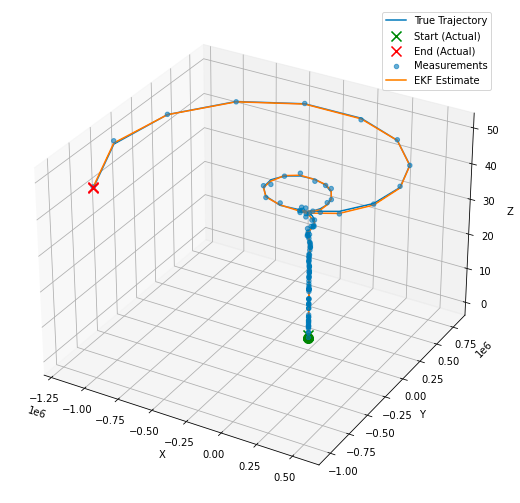
Building on our last Python example I have presented the implementation of the EKF:
import numpy as np
import matplotlib.pyplot as plt
from mpl_toolkits.mplot3d import Axes3D

class ExtendedKalmanFilter:
    """
    An implementation of the Extended Kalman Filter (EKF).
    This filter is suitable for systems with non-linear dynamics by linearising
    the system model at each time step using the Jacobian.

    Attributes:
        state_transition (callable): The state transition function for the system.
        jacobian_F (callable): Function to compute the Jacobian of the state transition.
        H (np.ndarray): The observation matrix.
        jacobian_H (callable): Function to compute the Jacobian of the observation model.
        Q (np.ndarray): The process noise covariance matrix.
        R (np.ndarray): The measurement noise covariance matrix.
        x (np.ndarray): The initial state estimate.
        P (np.ndarray): The initial estimate covariance.
    """
    def __init__(self, state_transition, jacobian_F, observation_matrix, jacobian_H, Q, R, x, P):
        """
        Constructs the Extended Kalman Filter.

        Parameters:
            state_transition (callable): The state transition function.
            jacobian_F (callable): Function to compute the Jacobian of F.
            observation_matrix (np.ndarray): Observation matrix.
            jacobian_H (callable): Function to compute the Jacobian of H.
            Q (np.ndarray): Process noise covariance.
            R (np.ndarray): Measurement noise covariance.
            x (np.ndarray): Initial state estimate.
            P (np.ndarray): Initial estimate covariance.
        """
        self.state_transition = state_transition  # Non-linear state transition function
        self.jacobian_F = jacobian_F  # Function to compute Jacobian of F
        self.H = observation_matrix  # Observation matrix
        self.jacobian_H = jacobian_H  # Function to compute Jacobian of H
        self.Q = Q  # Process noise covariance
        self.R = R  # Measurement noise covariance
        self.x = x  # Initial state estimate
        self.P = P  # Initial estimate covariance

    def predict(self, u):
        """
        Predicts the state at the next time step.

        Parameters:
            u (np.ndarray): The control input vector.
        """
        self.x = self.state_transition(self.x, u)
        F = self.jacobian_F(self.x, u)
        self.P = F @ self.P @ F.T + self.Q

    def update(self, z):
        """
        Updates the state estimate with a new measurement.

        Parameters:
            z (np.ndarray): The measurement vector.
        """
        H = self.jacobian_H()
        y = z - self.H @ self.x
        S = H @ self.P @ H.T + self.R
        K = self.P @ H.T @ np.linalg.inv(S)
        self.x = self.x + K @ y
        self.P = (np.eye(len(self.x)) - K @ H) @ self.P

# Define the non-linear transition and Jacobian functions
def state_transition(x, u):
    """
    Defines the state transition function for the system with non-linear dynamics.

    Parameters:
        x (np.ndarray): The current state vector.
        u (np.ndarray): The control input vector containing time step and rate of change of angular velocity.

    Returns:
        np.ndarray: The next state vector as predicted by the state transition function.
    """
    dt = u[0]
    alpha = u[1]
    x_next = np.array([
        x[0] - x[3] * x[1] * dt,
        x[1] + x[3] * x[0] * dt,
        x[2] + x[3] * dt,
        x[3],
        x[4] + alpha * dt
    ])
    return x_next

def jacobian_F(x, u):
    """
    Computes the Jacobian matrix of the state transition function.

    Parameters:
        x (np.ndarray): The current state vector.
        u (np.ndarray): The control input vector containing time step and rate of change of angular velocity.

    Returns:
        np.ndarray: The Jacobian matrix of the state transition function at the current state.
    """
    dt = u[0]
    # Compute the Jacobian matrix of the state transition function
    F = np.array([
        [1, -x[3]*dt, 0, -x[1]*dt, 0],
        [x[3]*dt, 1, 0, x[0]*dt, 0],
        [0, 0, 1, dt, 0],
        [0, 0, 0, 1, 0],
        [0, 0, 0, 0, 1]
    ])
    return F

def jacobian_H():
    # Jacobian matrix for the observation function is simply the observation matrix
    return H

# Simulation parameters
num_steps = 100
dt = 1.0
alpha = 0.01  # Rate of change of angular velocity

# Observation matrix, assuming we can directly observe the x, y, and z position
H = np.eye(3, 5)

# Process noise covariance matrix
Q = np.diag([0.1, 0.1, 0.1, 0.1, 0.01])

# Measurement noise covariance matrix
R = np.diag([0.5, 0.5, 0.5])

# Initial state estimate and covariance
x0 = np.array([0, 20, 0, 0.5, 0.1])  # [x, y, z, v, omega]
P0 = np.eye(5)

# Instantiate the EKF
ekf = ExtendedKalmanFilter(state_transition, jacobian_F, H, jacobian_H, Q, R, x0, P0)

# Generate true trajectory and measurements
true_states = []
measurements = []
for t in range(num_steps):
    u = np.array([dt, alpha])
    true_state = state_transition(x0, u)  # This would be your true system model
    true_states.append(true_state)
    measurement = true_state[:3] + np.random.multivariate_normal(np.zeros(3), R)  # Simulate measurement noise
    measurements.append(measurement)
    x0 = true_state  # Update the true state

# Now we run the EKF over the measurements
estimated_states = []
for z in measurements:
    ekf.predict(u=np.array([dt, alpha]))
    ekf.update(z=np.array(z))
    estimated_states.append(ekf.x)

# Convert lists to arrays for plotting
true_states = np.array(true_states)
measurements = np.array(measurements)
estimated_states = np.array(estimated_states)

# Plotting the results
fig = plt.figure(figsize=(12, 9))
ax = fig.add_subplot(111, projection='3d')

# Plot the true trajectory
ax.plot(true_states[:, 0], true_states[:, 1], true_states[:, 2], label='True Trajectory')
# Increase the size of the start and end markers for the true trajectory
ax.scatter(true_states[0, 0], true_states[0, 1], true_states[0, 2], label='Start (Actual)', c='green', marker='x', s=100)
ax.scatter(true_states[-1, 0], true_states[-1, 1], true_states[-1, 2], label='End (Actual)', c='red', marker='x', s=100)

# Plot the measurements
ax.scatter(measurements[:, 0], measurements[:, 1], measurements[:, 2], label='Measurements', alpha=0.6)
# Plot the start and end markers for the measurements
ax.scatter(measurements[0, 0], measurements[0, 1], measurements[0, 2], c='green', marker='o', s=100)
ax.scatter(measurements[-1, 0], measurements[-1, 1], measurements[-1, 2], c='red', marker='x', s=100)

# Plot the EKF estimate
ax.plot(estimated_states[:, 0], estimated_states[:, 1], estimated_states[:, 2], label='EKF Estimate')


ax.set_xlabel('X')
ax.set_ylabel('Y')
ax.set_zlabel('Z')
ax.legend()

plt.show()
A simple summary
In this blog we have explored in depth how to build and apply a Kalman Filter (KF), as well as covering how to implement an Extended Kalman Filter (EKF). Let’s end by summarising the use cases, advantages and disadvantages of these models.
KF: This model is applicable to linear systems, where we can assume that the state transitions and obeservation matrices are linear functions of the state (with some gaussian noise). You might consider applying this algorithm for:
- tracking the position and velocity of an object moving at a constant speed
- signal processing applications if the noise is stochastic or can be represented by linear models
- economic forecasting if the underlining relationships can be modelled linearly
The key advantage for the KF is that (once you follow the matrix calculations) the algorithm is quite simple, computationally less intensive than other approaches and can provide very accurate forecasts and estimations of the true state of the system in time. The disadvantage is the assumption of linearity which typically does not hold true in complex real-world scenarios.
EKF: We can essentially consider the EKF as the nonlinear equivalent of the KF, supported by the use of the Jacobian. You would consider the EKF if you are dealing with:
- robotic systems where the measurement and system dynamics are typically nonlinear
- tracking and navigation systems that often involve non-constant velocities or changes in angular rate such as that from tracking aircrafts or spacecrafts.
- automotive systems when implementing cruise control or lane-keeping that is found in the most modern ‘smart’ cars.
The EKF often produces better estimates that the KF, in particular for nonlinear systems, however it can become far more computationally intensive due to the calculation of the Jacobian matrix. This approach also relies on first-order linear approximations from the Taylor series expansion, which might not be an appropriate assumption for highly nonlinear systems. The addition of the Jacobian can also make the model more challenging to design and as such despite its advantages it may be more appropriate to implement the KF for simplicity and interoperability.
Unless otherwise noted, all images are by the author.
Exposing the Power of the Kalman Filter was originally published in Towards Data Science on Medium, where people are continuing the conversation by highlighting and responding to this story.
Denial of responsibility! Techno Blender is an automatic aggregator of the all world’s media. In each content, the hyperlink to the primary source is specified. All trademarks belong to their rightful owners, all materials to their authors. If you are the owner of the content and do not want us to publish your materials, please contact us by email – [email protected]. The content will be deleted within 24 hours.