
Feature Engineering for Machine Learning with Picture Data | by Anthony Cavin | Jun, 2022
Fight the curse of dimensionality
Feature engineering is the process of taking raw data and extracting features that are useful for modeling. With images, this usually means extracting things like color, texture, and shape. There are many ways to do feature engineering, and the approach you take will depend on the type of data you’re working with and the problem you’re trying to solve.
But why would we need it with images?
Images encapsulate a lot of information but that comes at a cost: high dimensionality. For instance, a small picture of size 200 by 100 pixels with 3 channels (red, green, blue) already represents a feature vector with 60’000 dimensions.
That’s a lot to handle, and we are facing the curse of dimensionality. We will speak a bit more about that later.

In this post, we’ll take a look at how we can reduce the dimension of a picture to fight the curse of dimensionality.
The “curse of dimensionality” is a term used to describe the problems that arise when working with datasets that have a large number of dimensions.
One reason is that the number of data points needed to accurately learn the underlying distribution of the data increases exponentially with the number of dimensions. In other words, if we have a data set with 100 features, we might need around 1,000 or even 10,000 data points to have a good chance of accurately learning.
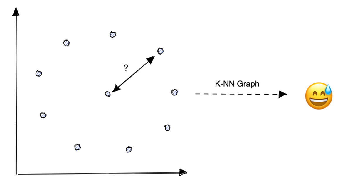
To better understand the curse of dimensionality, I like to take the example of a k-nearest neighbor graph in two dimensions as in the picture below.

But what happens if all points are equidistant to each other? This is a very unlikely scenario, but it shows (to some extent) what is typically happening when we try to compute the euclidian distance between features that have a lot of dimensions.
To understand how the number of dimensions affects our distance metric, we can have a look at the ratio between the volume inside and outside an n-dimensional ball (n-ball) inscribed in a hypercube.

We can observe in this graph that the volume outside the n-ball will take the majority of the space. This is very counterintuitive and does not resemble the two- or three-dimensional space we are used to mastering.
If we evenly distribute points in a hypercube, it’s very unlikely that any of them would fall inside the inscribed n-ball.
This would give the impression that all points in the hypercube will be very far from the center of the n-ball and would look equidistance and concentrated in long spiky corners of the hypercube. This will cause our distance-based algorithms to be susceptible to noise on the input features.
So, how can we solve it?
A simple way to reduce the dimension of our feature vector is to decrease the size of the image with decimation (downsampling) by reducing the resolution of the image.
If the color component is not relevant, we can also convert pictures to grayscale to divide the number dimension by three. But there are other ways to reduce the dimension of the picture and potentially extract features. For example, we can use wavelet decomposition.
Wavelet decomposition is a way of breaking down a signal in both space and frequency. In the case of pictures, this means breaking down the image into its horizontal, vertical, and diagonal components.

The HOG feature descriptor is a popular technique used in computer vision and image processing for detecting objects in digital images. The HOG descriptor became popular after Dalal and Triggs showed the efficiency of this descriptor in 2005 that focused on pedestrian detection in static images.
The HOG descriptor is a type of feature descriptor that encodes the shape and appearance of an object by computing the distribution of intensity gradients in an image.
The most important parameter in our case is the number of pixels per cell as it will give us a way to find the best trade-off between the number of dimensions and the number of details captured in the picture.


For the example above, the input image has 20,000 dimensions (100 by 200 pixels) and the HOG feature has 2,400 dimensions with the 8 by 8-pixel cell and 576 for the 16 by 16-pixel cell. That’s an 88% and 97% reduction, respectively.
We can also use Principal Component Analysis (PCA) to reduce the dimension of our feature vector. PCA is a statistical technique that can be used to find the directions (components) that maximize the variance and minimizes the projection error in a dataset.

In other words, PCA can be used to find the directions that represent the most information in the data.
There are a few things to keep in mind when using PCA:
- PCA is best used as a tool for dimensionality reduction, not for feature selection.
- When using PCA for dimensionality reduction, it is important to normalize the data first.
- PCA is a linear transformation, so it will not be able to capture non-linear relationships in the data.
- To reduce to N dimensions, you need at least N-1 observations
I recommend reading the following article to better understand PCA and its limitations:
Manifold Learning is in some ways an extension of linear methods like PCA to reduce dimensionality but for non-linear structures in data.
A manifold is a topological space that is locally Euclidean, meaning that near each point it resembles the Euclidean space. Manifolds appear naturally in many areas of mathematics and physics, and the study of manifolds is a central topic in differential geometry.
There are a few things to keep in mind when working with manifold learning:
- Manifold learning is a powerful tool for dimensionality reduction.
- It can be used to find hidden patterns in data.
- Manifold learning is usually a computationally intensive task, so it is important to have a good understanding of the algorithms before using them.
It’s very rare that a real-life process uses all of its dimensions to describe its underlying structure. For example with the pictures below, only a few dimensions should be necessary to describe the cup’s position and rotation.

And that’s the case, once projected with a manifold learning algorithm such as t-distributed Stochastic Neighbor Embedding (t-SNE), only two dimensions are able to encode the cup position and rotation.
Encoded position:

Encoded rotation:

In this post, we’ve seen how to use feature engineering with pictures to fight the curse of dimensionality. We’ve looked at how to reduce the dimension of a picture with decimation, wavelet decomposition, the HOG descriptor, and PCA. We’ve also seen how to use manifold learning to find hidden patterns in data.
There are many other ways to reduce the dimension of a picture, and the approach you take will depend on the type of data you’re working with and the problem you’re trying to solve.
Feature engineering is an iterative process, and it helps to have an overview of different possibilities and available approaches.
I hope you found this post helpful! If you have any questions about how to build the k-NN graph, I suggest reading the following article:
Fight the curse of dimensionality

Feature engineering is the process of taking raw data and extracting features that are useful for modeling. With images, this usually means extracting things like color, texture, and shape. There are many ways to do feature engineering, and the approach you take will depend on the type of data you’re working with and the problem you’re trying to solve.
But why would we need it with images?
Images encapsulate a lot of information but that comes at a cost: high dimensionality. For instance, a small picture of size 200 by 100 pixels with 3 channels (red, green, blue) already represents a feature vector with 60’000 dimensions.
That’s a lot to handle, and we are facing the curse of dimensionality. We will speak a bit more about that later.
In this post, we’ll take a look at how we can reduce the dimension of a picture to fight the curse of dimensionality.
The “curse of dimensionality” is a term used to describe the problems that arise when working with datasets that have a large number of dimensions.
One reason is that the number of data points needed to accurately learn the underlying distribution of the data increases exponentially with the number of dimensions. In other words, if we have a data set with 100 features, we might need around 1,000 or even 10,000 data points to have a good chance of accurately learning.
To better understand the curse of dimensionality, I like to take the example of a k-nearest neighbor graph in two dimensions as in the picture below.
But what happens if all points are equidistant to each other? This is a very unlikely scenario, but it shows (to some extent) what is typically happening when we try to compute the euclidian distance between features that have a lot of dimensions.
To understand how the number of dimensions affects our distance metric, we can have a look at the ratio between the volume inside and outside an n-dimensional ball (n-ball) inscribed in a hypercube.
We can observe in this graph that the volume outside the n-ball will take the majority of the space. This is very counterintuitive and does not resemble the two- or three-dimensional space we are used to mastering.
If we evenly distribute points in a hypercube, it’s very unlikely that any of them would fall inside the inscribed n-ball.
This would give the impression that all points in the hypercube will be very far from the center of the n-ball and would look equidistance and concentrated in long spiky corners of the hypercube. This will cause our distance-based algorithms to be susceptible to noise on the input features.
So, how can we solve it?
A simple way to reduce the dimension of our feature vector is to decrease the size of the image with decimation (downsampling) by reducing the resolution of the image.
If the color component is not relevant, we can also convert pictures to grayscale to divide the number dimension by three. But there are other ways to reduce the dimension of the picture and potentially extract features. For example, we can use wavelet decomposition.
Wavelet decomposition is a way of breaking down a signal in both space and frequency. In the case of pictures, this means breaking down the image into its horizontal, vertical, and diagonal components.
The HOG feature descriptor is a popular technique used in computer vision and image processing for detecting objects in digital images. The HOG descriptor became popular after Dalal and Triggs showed the efficiency of this descriptor in 2005 that focused on pedestrian detection in static images.
The HOG descriptor is a type of feature descriptor that encodes the shape and appearance of an object by computing the distribution of intensity gradients in an image.
The most important parameter in our case is the number of pixels per cell as it will give us a way to find the best trade-off between the number of dimensions and the number of details captured in the picture.
For the example above, the input image has 20,000 dimensions (100 by 200 pixels) and the HOG feature has 2,400 dimensions with the 8 by 8-pixel cell and 576 for the 16 by 16-pixel cell. That’s an 88% and 97% reduction, respectively.
We can also use Principal Component Analysis (PCA) to reduce the dimension of our feature vector. PCA is a statistical technique that can be used to find the directions (components) that maximize the variance and minimizes the projection error in a dataset.
In other words, PCA can be used to find the directions that represent the most information in the data.
There are a few things to keep in mind when using PCA:
- PCA is best used as a tool for dimensionality reduction, not for feature selection.
- When using PCA for dimensionality reduction, it is important to normalize the data first.
- PCA is a linear transformation, so it will not be able to capture non-linear relationships in the data.
- To reduce to N dimensions, you need at least N-1 observations
I recommend reading the following article to better understand PCA and its limitations:
Manifold Learning is in some ways an extension of linear methods like PCA to reduce dimensionality but for non-linear structures in data.
A manifold is a topological space that is locally Euclidean, meaning that near each point it resembles the Euclidean space. Manifolds appear naturally in many areas of mathematics and physics, and the study of manifolds is a central topic in differential geometry.
There are a few things to keep in mind when working with manifold learning:
- Manifold learning is a powerful tool for dimensionality reduction.
- It can be used to find hidden patterns in data.
- Manifold learning is usually a computationally intensive task, so it is important to have a good understanding of the algorithms before using them.
It’s very rare that a real-life process uses all of its dimensions to describe its underlying structure. For example with the pictures below, only a few dimensions should be necessary to describe the cup’s position and rotation.
And that’s the case, once projected with a manifold learning algorithm such as t-distributed Stochastic Neighbor Embedding (t-SNE), only two dimensions are able to encode the cup position and rotation.
Encoded position:
Encoded rotation:
In this post, we’ve seen how to use feature engineering with pictures to fight the curse of dimensionality. We’ve looked at how to reduce the dimension of a picture with decimation, wavelet decomposition, the HOG descriptor, and PCA. We’ve also seen how to use manifold learning to find hidden patterns in data.
There are many other ways to reduce the dimension of a picture, and the approach you take will depend on the type of data you’re working with and the problem you’re trying to solve.
Feature engineering is an iterative process, and it helps to have an overview of different possibilities and available approaches.
I hope you found this post helpful! If you have any questions about how to build the k-NN graph, I suggest reading the following article:
Denial of responsibility! Techno Blender is an automatic aggregator of the all world’s media. In each content, the hyperlink to the primary source is specified. All trademarks belong to their rightful owners, all materials to their authors. If you are the owner of the content and do not want us to publish your materials, please contact us by email – [email protected]. The content will be deleted within 24 hours.