Feature Selection with Simulated Annealing in Python, Clearly Explained | by Kenneth Leung | Aug, 2022

The term ‘annealing’ comes from the field of materials science. It is a process where materials like metal or glass are heated and held at a hot temperature, before being cooled slowly in a controlled manner.

The purpose of annealing is to introduce favourable physical properties (e.g., ductility) into the material for smoother downstream manufacturing.

The heat causes random rearrangement of atoms in the material, leading to the removal of the weak connections and residual stress within.

The subsequent cooling settles the material and secures the desirable physical properties.

So how is this seemingly unrelated physical annealing linked with feature selection? You will be surprised to discover that simulated annealing is a global search method that mimics how annealing works.

In the context of feature selection, simulated annealing finds the subset of features that gives the best predictive model performance amongst the many possible subset combinations.

This idea is like how physical annealing aims to generate high-performing physical properties for the material.

To envision how simulated annealing relates to physical annealing, we can imagine the following comparisons:

• A material particle → A feature
• The material itself → Full set of features
• The current state of particle arrangement → Selected feature subset
• Change in material’s physical properties → Change in model performance

The repeated ‘heating’ and ‘cooling’ phases in simulated annealing help us find the best global subset of features.

Here is what the heating and cooling phases mean in the algorithm:

• Heating: Randomly alter the subset of features, evaluate change in model performance, and set a high probability of accepting a poorer performing subset over a better one. This phase is considered ‘exploration’.
• Cooling: Gradually reduce the probability of keeping poor-performing subsets so that high-performing subsets are increasingly likely to be kept. This phase is considered ‘exploitation’.

The rationale is that the initial heating lets the algorithm freely explore the search space. As the cooling begins, the algorithm is incentivized to exploit and home in on the global best feature subset.

Pros

Amongst the three common feature selection classes (i.e., intrinsic, filter, wrapper), wrapper methods are highly popular because they search a wider variety of feature subsets compared to the other two. However, the downside is that these wrapper methods are greedy approaches.

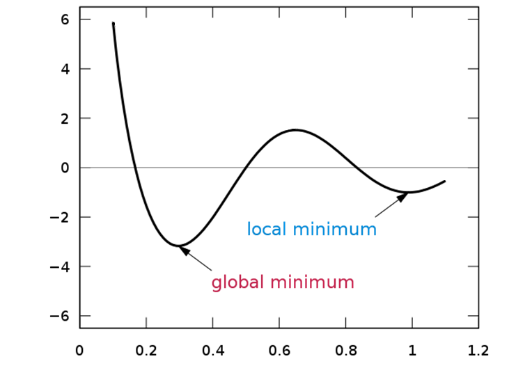
Greedy approaches choose search paths by going for the best immediate benefit at the time of each step at the expense of possible long-term gain. The result is that the search may get stuck at local optima.

On the contrary, simulated annealing is a probabilistic global optimization method that takes a non-greedy approach driven by the randomness imparted in the algorithm.

A non-greedy approach can to reassess previous subsets and can move in a direction that is initially unfavourable if there appears to be a potential benefit in the long run.

As a result, simulated annealing has a greater ability in escaping local optima and finding the global best subset of features.

Furthermore, its non-greedy nature creates a higher probability of capturing key feature interactions, especially if these interactions are significant only if the features co-occur in a subset.

Cons

A major disadvantage is that simulated annealing is computationally intensive, as you will see in the algorithm details later.

Therefore, it is best to first leverage domain knowledge to narrow down the overall set of features. With a smaller feature set to start with, it becomes more efficient to use simulated annealing for further feature selection.

Another disadvantage is that there are numerous algorithm parameters to tune, which can prove to be challenging.

Note: You may refer to the codes and data for this demo in this GitHub repo.

(i) Overview

To make the algorithm easier to understand, let’s break it down step by step and pair it with examples.

To contextualize the algorithm, we will be building a binary classifier with a random forest model on the Titanic dataset (to predict passenger survival) and with the ROC-AUC score as the performance metric.

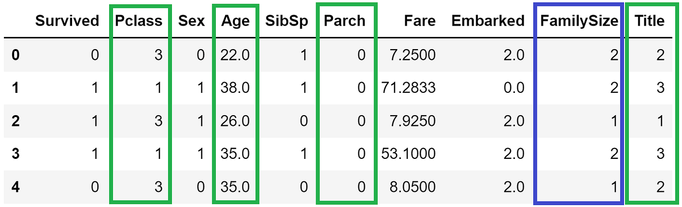
The pre-processed training data has a total of nine predictor features and a binary target variable (Survived).

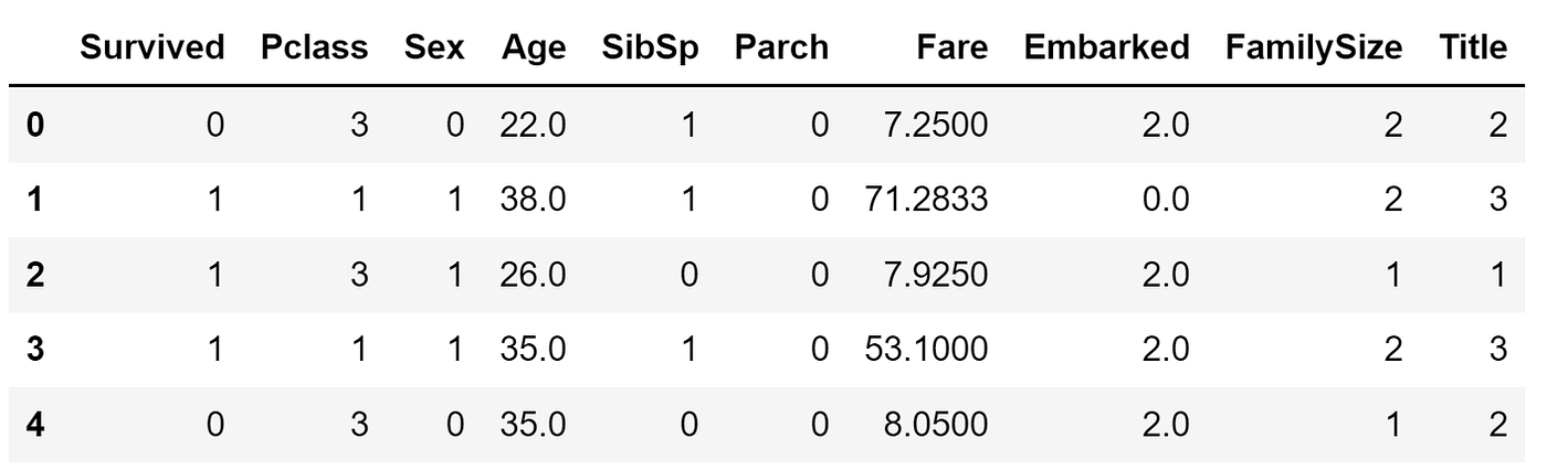
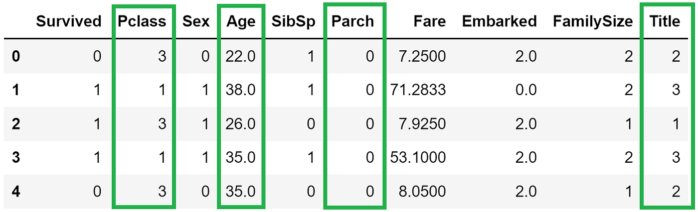
STEP 1 — Generate a random initial subset of features to form the current state. This can be done arbitrarily by randomly selecting 50% of the original features.

For example, let’s say our initial random subset of four features are Pclass, Age, Parch, and Title.

STEP 2 — Specify the maximum number of iterations to run. This is a tunable parameter, but we can start with an integer (e.g., 50) for simplicity.

STEP 3 — Evaluate model performance on the current subset to get an initial performance metric. For this case, we train a random forest classifier on the data filtered to the current 4-feature subset (Pclass, Age, Parch, Title) and retrieve the cross-validated AUC score.

The following steps (Steps 4 to 7) represent a single iteration. The maximum number of iterations to run is already defined in Step 2.

STEP 4 — Randomly alter the list of features in the current subset to generate a new subset by adding, replacing, or removing one feature.

For example, a random alteration generated a new 5-feature subset that now includes FamilySize.

Note: If a subset has already been visited before, we repeat this step until a new unseen subset is generated.

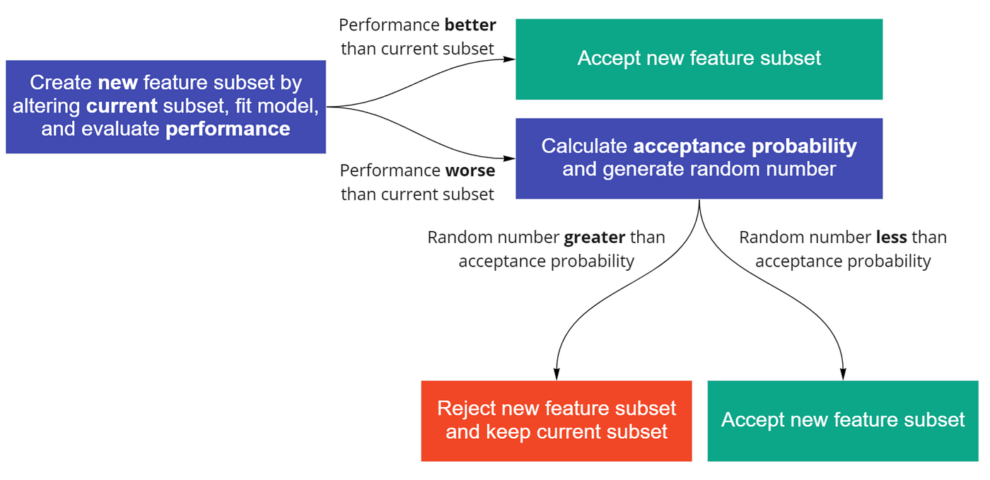
STEP 5 — Run the model on the new subset and compare the performance metric (i.e., AUC score) against that of the current subset.

STEP 6 — If the new subset performance is better, accept and update the new subset as the current state and end the iteration. If the performance is worse, continue to Step 7.

STEP 7 — Evaluate whether to accept the worse-performing new subset by first calculating an acceptance probability (more details later). Next, generate a random number uniformly in the range [0, 1].

If the random number is larger than the acceptance probability, reject the new subset and keep the current subset. Otherwise, accept and update the new subset as the current state.

At the end of each iteration, the acceptance probability is adjusted to establish a ‘cooling’ schedule. Let us see how this really works.

(ii) Acceptance Probability

We saw earlier (in Step 7) how the acceptance probability was used to decide whether to accept a poorer-performing new subset (and thereby make a non-improving move).

The acceptance probability is calculated as follows:

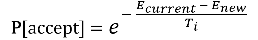
• The E terms refer to the performance metrics i.e., AUC scores. Enew is the cross-validated AUC score from the model trained on the new subset, while Ecurrent is based on the current subset. The difference between these two terms gives the change in model performance.
• Tᵢ represents the temperature at iteration i. Although the initial temperature (Tₒ) is tunable, we can start by setting it to a default high (maximum) value of 1 to initiate the heating phase.
• As the algorithm progresses, the temperature should cool and be reduced from the initial Tₒ. A popular strategy is geometric reduction where the temperature is scaled by a cooling factor alpha (α) after each iteration. The α value can be set by default as 0.95 since the typical range for α is between 0.95 and 0.99.

Here are how the parameters influence acceptance probability:

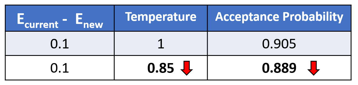
• As temperature decreases, the acceptance probability decreases. It means that there is a higher chance for the random number to be larger than the acceptance probability. It implies that we are more likely to reject the poor-performing new subset.

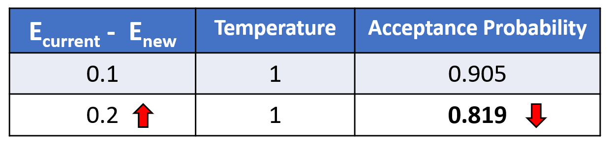
• As the new subset model performance worsens to a larger degree (i.e., a bigger difference between Ecurrent and Enew), the acceptance probability decreases. Likewise, it means we are more likely to reject the poor-performing new subset.

The controlled decrease from high to low temperature allows poor solutions to have a higher probability of acceptance early in the search but are more likely to be rejected later.

(iii) Termination Conditions

It would also be useful to include termination conditions (aka stopping criteria) so that the algorithm does not iterate needlessly.

Some examples of termination conditions include:

• Reaching an acceptable performance threshold
• Reaching a specific end temperature (e.g., T=0.01)
• Hitting a pre-determined number of successive iterations without performance improvement

(iv) Algorithm Pseudocode

An online search for simulated annealing will yield a multitude of intimidating pseudocodes to represent the algorithm. Here is an example:

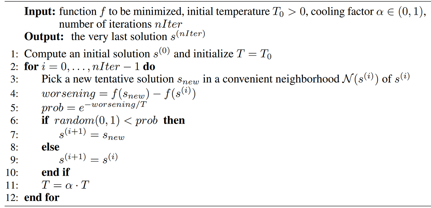
With the explanations in the earlier sections, you are now well-poised to appreciate and understand such codes regardless of the symbols and abbreviations used.

With the theoretical concepts established, let‘s see how to put simulated annealing into practice.

Here is the code for implementing the algorithm in Python. You can also view the full Python script here.

The function train_model above runs a random forest classifier with 3-fold cross-validation to obtain an AUC score.

Feel free to check out this notebook to see the complete output.

Upon running the simulated annealing function on the Titanic dataset, we obtain results that look like this:

We can observe that the best AUC score obtained is 0.867, which corresponds to iteration 4 with the feature set of [0,1,2,5,8]. When the indices are mapped to the column names, the five features are Pclass, Sex, Age, Fare, and Title.

A caveat is that this implementation assumes that a higher metric score relates to better performance (e.g., AUC, Accuracy). However, if we use metrics like RMSE where lower scores are better, the inequality signs need to be inversed accordingly e.g., metric < prev_metric instead of metric > prev_metric.

While R has an established package (caret) to run simulated annealing, Python seems to be lacking such a solution. If you know of any Python package that does feature selection with simulated annealing, do let me know!

So far, we have walked through the concepts and basic implementation of simulated annealing for feature selection in Python.

You will be glad to know that there are advanced implementations available to make the algorithm more robust.

One example is the concept of restarts, where the search resets to the last known optimal solution if a new optimal solution is not found after n iterations. Its purpose is to provide an extra layer of protection to prevent the search from lingering in poor-performing local optima.

The GitHub repo for this project can be found here, along with the references. As always, I look forward to your feedback on this topic!

I welcome you to join me on a data science learning journey! Follow this Medium page and check out my GitHub to stay in the loop of more exciting data science content. Meanwhile, have fun running simulated annealing for feature selection!

The term ‘annealing’ comes from the field of materials science. It is a process where materials like metal or glass are heated and held at a hot temperature, before being cooled slowly in a controlled manner.

The purpose of annealing is to introduce favourable physical properties (e.g., ductility) into the material for smoother downstream manufacturing.

The heat causes random rearrangement of atoms in the material, leading to the removal of the weak connections and residual stress within.

The subsequent cooling settles the material and secures the desirable physical properties.

So how is this seemingly unrelated physical annealing linked with feature selection? You will be surprised to discover that simulated annealing is a global search method that mimics how annealing works.

In the context of feature selection, simulated annealing finds the subset of features that gives the best predictive model performance amongst the many possible subset combinations.

This idea is like how physical annealing aims to generate high-performing physical properties for the material.

To envision how simulated annealing relates to physical annealing, we can imagine the following comparisons:

• A material particle → A feature
• The material itself → Full set of features
• The current state of particle arrangement → Selected feature subset
• Change in material’s physical properties → Change in model performance

The repeated ‘heating’ and ‘cooling’ phases in simulated annealing help us find the best global subset of features.

Here is what the heating and cooling phases mean in the algorithm:

• Heating: Randomly alter the subset of features, evaluate change in model performance, and set a high probability of accepting a poorer performing subset over a better one. This phase is considered ‘exploration’.
• Cooling: Gradually reduce the probability of keeping poor-performing subsets so that high-performing subsets are increasingly likely to be kept. This phase is considered ‘exploitation’.

The rationale is that the initial heating lets the algorithm freely explore the search space. As the cooling begins, the algorithm is incentivized to exploit and home in on the global best feature subset.

Pros

Amongst the three common feature selection classes (i.e., intrinsic, filter, wrapper), wrapper methods are highly popular because they search a wider variety of feature subsets compared to the other two. However, the downside is that these wrapper methods are greedy approaches.

Greedy approaches choose search paths by going for the best immediate benefit at the time of each step at the expense of possible long-term gain. The result is that the search may get stuck at local optima.

On the contrary, simulated annealing is a probabilistic global optimization method that takes a non-greedy approach driven by the randomness imparted in the algorithm.

A non-greedy approach can to reassess previous subsets and can move in a direction that is initially unfavourable if there appears to be a potential benefit in the long run.

As a result, simulated annealing has a greater ability in escaping local optima and finding the global best subset of features.

Furthermore, its non-greedy nature creates a higher probability of capturing key feature interactions, especially if these interactions are significant only if the features co-occur in a subset.

Cons

A major disadvantage is that simulated annealing is computationally intensive, as you will see in the algorithm details later.

Therefore, it is best to first leverage domain knowledge to narrow down the overall set of features. With a smaller feature set to start with, it becomes more efficient to use simulated annealing for further feature selection.

Another disadvantage is that there are numerous algorithm parameters to tune, which can prove to be challenging.

Note: You may refer to the codes and data for this demo in this GitHub repo.

(i) Overview

To make the algorithm easier to understand, let’s break it down step by step and pair it with examples.

To contextualize the algorithm, we will be building a binary classifier with a random forest model on the Titanic dataset (to predict passenger survival) and with the ROC-AUC score as the performance metric.

The pre-processed training data has a total of nine predictor features and a binary target variable (Survived).

STEP 1 — Generate a random initial subset of features to form the current state. This can be done arbitrarily by randomly selecting 50% of the original features.

For example, let’s say our initial random subset of four features are Pclass, Age, Parch, and Title.

STEP 2 — Specify the maximum number of iterations to run. This is a tunable parameter, but we can start with an integer (e.g., 50) for simplicity.

STEP 3 — Evaluate model performance on the current subset to get an initial performance metric. For this case, we train a random forest classifier on the data filtered to the current 4-feature subset (Pclass, Age, Parch, Title) and retrieve the cross-validated AUC score.

The following steps (Steps 4 to 7) represent a single iteration. The maximum number of iterations to run is already defined in Step 2.

STEP 4 — Randomly alter the list of features in the current subset to generate a new subset by adding, replacing, or removing one feature.

For example, a random alteration generated a new 5-feature subset that now includes FamilySize.

Note: If a subset has already been visited before, we repeat this step until a new unseen subset is generated.

STEP 5 — Run the model on the new subset and compare the performance metric (i.e., AUC score) against that of the current subset.

STEP 6 — If the new subset performance is better, accept and update the new subset as the current state and end the iteration. If the performance is worse, continue to Step 7.

STEP 7 — Evaluate whether to accept the worse-performing new subset by first calculating an acceptance probability (more details later). Next, generate a random number uniformly in the range [0, 1].

If the random number is larger than the acceptance probability, reject the new subset and keep the current subset. Otherwise, accept and update the new subset as the current state.

At the end of each iteration, the acceptance probability is adjusted to establish a ‘cooling’ schedule. Let us see how this really works.

(ii) Acceptance Probability

We saw earlier (in Step 7) how the acceptance probability was used to decide whether to accept a poorer-performing new subset (and thereby make a non-improving move).

The acceptance probability is calculated as follows:

• The E terms refer to the performance metrics i.e., AUC scores. Enew is the cross-validated AUC score from the model trained on the new subset, while Ecurrent is based on the current subset. The difference between these two terms gives the change in model performance.
• Tᵢ represents the temperature at iteration i. Although the initial temperature (Tₒ) is tunable, we can start by setting it to a default high (maximum) value of 1 to initiate the heating phase.
• As the algorithm progresses, the temperature should cool and be reduced from the initial Tₒ. A popular strategy is geometric reduction where the temperature is scaled by a cooling factor alpha (α) after each iteration. The α value can be set by default as 0.95 since the typical range for α is between 0.95 and 0.99.

Here are how the parameters influence acceptance probability:

• As temperature decreases, the acceptance probability decreases. It means that there is a higher chance for the random number to be larger than the acceptance probability. It implies that we are more likely to reject the poor-performing new subset.

• As the new subset model performance worsens to a larger degree (i.e., a bigger difference between Ecurrent and Enew), the acceptance probability decreases. Likewise, it means we are more likely to reject the poor-performing new subset.

The controlled decrease from high to low temperature allows poor solutions to have a higher probability of acceptance early in the search but are more likely to be rejected later.

(iii) Termination Conditions

It would also be useful to include termination conditions (aka stopping criteria) so that the algorithm does not iterate needlessly.

Some examples of termination conditions include:

• Reaching an acceptable performance threshold
• Reaching a specific end temperature (e.g., T=0.01)
• Hitting a pre-determined number of successive iterations without performance improvement

(iv) Algorithm Pseudocode

An online search for simulated annealing will yield a multitude of intimidating pseudocodes to represent the algorithm. Here is an example:

With the explanations in the earlier sections, you are now well-poised to appreciate and understand such codes regardless of the symbols and abbreviations used.

With the theoretical concepts established, let‘s see how to put simulated annealing into practice.

Here is the code for implementing the algorithm in Python. You can also view the full Python script here.

The function train_model above runs a random forest classifier with 3-fold cross-validation to obtain an AUC score.

Feel free to check out this notebook to see the complete output.

Upon running the simulated annealing function on the Titanic dataset, we obtain results that look like this:

We can observe that the best AUC score obtained is 0.867, which corresponds to iteration 4 with the feature set of [0,1,2,5,8]. When the indices are mapped to the column names, the five features are Pclass, Sex, Age, Fare, and Title.

A caveat is that this implementation assumes that a higher metric score relates to better performance (e.g., AUC, Accuracy). However, if we use metrics like RMSE where lower scores are better, the inequality signs need to be inversed accordingly e.g., metric < prev_metric instead of metric > prev_metric.

While R has an established package (caret) to run simulated annealing, Python seems to be lacking such a solution. If you know of any Python package that does feature selection with simulated annealing, do let me know!

So far, we have walked through the concepts and basic implementation of simulated annealing for feature selection in Python.

You will be glad to know that there are advanced implementations available to make the algorithm more robust.

One example is the concept of restarts, where the search resets to the last known optimal solution if a new optimal solution is not found after n iterations. Its purpose is to provide an extra layer of protection to prevent the search from lingering in poor-performing local optima.

The GitHub repo for this project can be found here, along with the references. As always, I look forward to your feedback on this topic!

I welcome you to join me on a data science learning journey! Follow this Medium page and check out my GitHub to stay in the loop of more exciting data science content. Meanwhile, have fun running simulated annealing for feature selection!