
Five Killer Optimization Techniques Every Pandas User Should Know | by Avi Chawla | Jul, 2022
A step towards data analysis run-time optimization
The motivation to design and build real-world applicable machine learning models has always intrigued Data Scientists to leverage optimized, efficient, and accurate methods at scale. Optimization plays a foundational role in sustainably delivering real-world and user-facing software solutions.
While I understand that not everyone is building solutions at scale, awareness about various optimization and time-saving techniques is nevertheless helpful and highly applicable to even generic Data Science/Machine Learning use-cases.
Therefore, in this post, I will introduce you to a handful of incredible techniques to reduce the run-time of your regular tabular data analysis, management, and processing tasks using Pandas. To get a brief overview, I will discuss the following topics in this post:
#1 Input/Output on CSV
#2 Filtering Based on Categorical data
#3 Merging DataFrames
#4 Value_counts() vs GroupBy()
#5 Iterating over a DataFrame
Moreover, you can get the notebook for this post here.
Let’s begin 🚀!
CSV files are by far the most prevalent source to read DataFrames from and store DataFrames to, aren’t they? This is because CSVs provide tremendous flexibility in the context of input and output operation using the pd.read_csv() and df.to_csv() method such as:
- CSVs can be opened in Excel and manipulated in every way Excel allows you to.
- CSVs enable you to read only a subset of columns if needed by specifying the columns as a list and passing it as the
usecolsargument ofpd.read_csv()method. - You can read only the first
nrows if needed using thenrowsargument of thepd.read_csv()method, etc.
While I admit that there are numerous advantages of using CSV files, at the same time, they are far from being the go-to method if you are looking for run-time optimization. Let me explain.
Input-output operations with Pandas to a CSV file are serialized, inevitably making them highly inefficient and time-consuming. While there is ample scope to parallelize stuff, Pandas, unfortunately, does not have this functionality (yet).
Till then, if you are stuck with reading CSV files, there are two incredibly faster alternatives you can take, which I have depicted in the flow chart below:
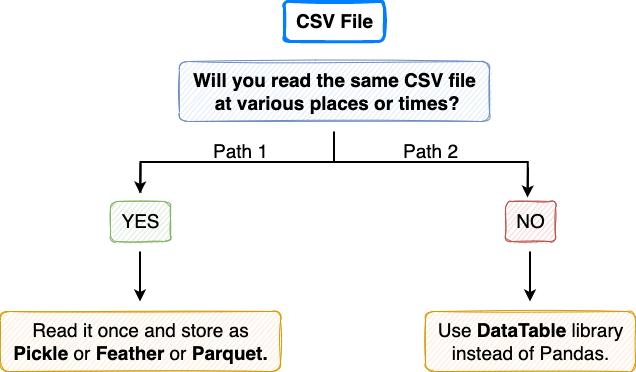
Path 1
If your CSV file is static and you think you will read it multiple times, possibly in the same pipeline or after reloading the kernel, immediately save it as a Pickle or Feather or a Parquet file. But Why? This I have already discussed in my post below:
This conversion from CSV format to your desired alternative is demonstrated in the code block below:
Now, when you want to read the DataFrame back, instead of reading it from the CSV file, read it using the new file you created. The corresponding methods in Pandas to reload the dataset is shown below:
Moreover, each of these individual files will interpret the records as a Pandas DataFrame. This can be verified using the type() method in Python as follows:
The bar-plot below depicts the expected speed up in the run-time for all the four individual file formats:

To obtain the run-time of the four formats, I generated a random dataset in Python with a million rows and thirty columns — encompassing string, float, and integer data types. I measured the load and the save run-time ten times to reduce randomness and draw fair conclusions from the observed results. The results above indicate averages across the ten experiments.
Path 2
If your CSV file isn’t static or you are going to use the CSV file just once, conversion to a new format does not make sense. Instead, take Path 2, i.e., use the DataTable library for input and output operations. You can install DataTable using the following command in a Jupyter Notebook:
When using DataTable, the CSV file will be interpreted as a DataTable DataFrame, not the Pandas DataFrame. Therefore, after loading the CSV file, you need to convert it to Pandas DataFrame. I have implemented this below:
Similarly, if you want to store a Pandas DataFrame to a CSV, prefer taking the DataTable route instead of Pandas. Here, to generate a CSV file using datatable, you first need to convert the Pandas DataFrame to a DataTable DataFrame and then store it in a CSV file. This is implemented below:
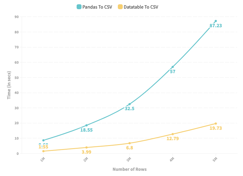
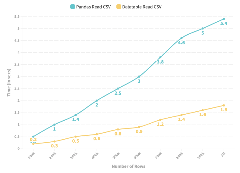
As depicted in the line chart above, DataTable provides high-speed input and output operations for a CSV file over a Pandas.
Key Takeaways/Final Thoughts
- If you are bound to use a CSV file due to some restrictions, never use the Pandas
read_csv()andto_csv()methods. Instead, prefer datatable’s input-output methods, as shown above. - If you will repeatedly read the same CSV file, convert it to one of Pickle, Feather, and Parquet, and then use the new file for input operations.
Data filtering is another common and widely-used operation in Pandas. The core idea is to select a segment of a dataframe that adheres to a specific condition.
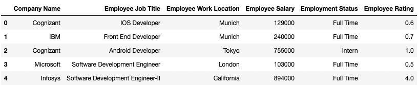
To demonstrate, consider a dummy DataFrame of over 4 million records I created myself. The first five rows are shown in the image below:
The code block below demonstrates my implementation:
Say you want to filter all the records which belong to “Amazon”. This can be done as follows:
Another way of doing the same filtering is by using groupby() and obtaining the individual group using the get_group() method as shown below:
The latter method provides speed-ups of up to 14 times as compared to the usual filtering method, which is a tremendous improvement in the run-time.
Moreover, the get_group() the method returns the individual group as a Pandas DataFrame. Therefore, you can proceed with the usual analysis post that. We can verify this by checking the type of dataframe obtained in Approach 1 and Approach 2 as follows:
Key Takeaways/Final Thoughts
- If you will perform repeated filtering of your DataFrame on categorical data, prefer grouping the data first using the
groupby()method. After that, fetch the desired groups using theget_group()method. - Caveat: This approach is only applicable to filtering based on categorical data.
Merge in Pandas refers to combining two DataFrames based on a join condition. This is similar to joins in Structured Query Language (SQL). You can execute merge using the pd.merge() method in Pandas as follows:
Although there is nothing wrong with the above method to link dataframes, there is a faster alternative available to join two dataframes using the join() method.
In the code block below, I have implemented the merge operation using the merge() method and the join() method. Here, we measure the time taken for the merge operation using the two methods.
With the join() method, we notice an improvement of over 4 times relative to the standard merge() method in Pandas.
Here, the join() method first expects you to change the index column and set it to the specific column on which you wish to execute joins between tables. This is done using the set_index() method in Pandas, as shown above.
If you want to execute a join condition on multiple columns, you can do that too using the join() method. First, pass the columns you wish to execute the join condition on as a list to the set_index() method. Then, call the join() method as before. This is demonstrated below:
Key Takeaways/Final Thoughts
- While performing joins, always change the index of both the DataFrames and set it to the column(s) you want to execute the join condition on.
We use value_counts() in Pandas to find the frequency of individual elements in a series. For instance, consider the dummy employee DataFrame we used in Section 2.
We can find the number of employees belonging to each company in this dataset using the value_counts() method as follows:
Similar frequency calculation can also be done using groupby(). The code below demonstrates that:
The output of value_counts() is arranged in descending order of frequencies. On the other hand, the output of size() on groupby() is sorted on the index column, which in this case is Company Name.
Assuming we are not bothered with how the output is arranged or sorted, we can measure the difference in run-time of the two methods to obtain the desired frequency as follows:
Even though both the methods essentially do the same thing (if we ignore the order of the output for once), there is a significant run-time difference between the two — groupby() being 1.5 times slower than value_counts().
Things get even worse when you want to obtain normalized frequencies, which denote the percentage/fraction of individual elements in the series. The run-time, in this case, is compared below:
Once again, although both the methods do the same thing, there is a significant run-time difference between the two — groupby() being close to 2 times slower than value_counts().
Key Takeaways/Final Thoughts
- For frequency-based measures, prefer using
value_counts()instead ofgroupby(). value_counts()can be used on multiple columns at once. Therefore, If you want to compute frequency on a combination of values from multiple columns, do that withvalue_counts()instead ofgroupby().
Looping or iterating over a DataFrame is the process of visiting every row individually and performing some pre-defined operations on the record. Although the best thing in such cases is to avoid looping altogether in the first place and prefer vectorized approaches, there might be situations where looping is necessary.
There are three methods in Pandas through which iteration is possible. Below, we’ll discuss them and compare their run-time on the employee dummy dataset used in the sections below. To revisit, the image below shows the first five rows of the DataFrame.
The three methods to loop over a DataFrame are:
- Iterate using
range(len(df)). - Iterate using
iterrows(). - Iterate using
itertuples().
I have implemented three functions in the code block below which utilize these three methods. The objective of the function is to calculate the mean salary of all employees in the DataFrame. We also find the run-time of each of these methods on the same DataFrame below.
Method 1: Iterate using range(len(df))
The average run-time to iterate over 4 million records is 46.1 ms.
Method 2: Iterate using iterrows()
The iterrows() method provides a substantial improvement in the iteration process, reducing the run-time by 2.5 times from 46.1 ms to 18.2 ms.
Method 3: Iterate using itertuples()
The itertuples() method turns out to be even better than iterrows(), reducing the run-time further by over 23 times from 18.2 ms to 773 µs.
Key Takeaways/Final Thoughts
- First, you should avoid introducing for-loops in your code to iterate over a DataFrame. Think of a vectorized solution if possible.
- If vectorization is not possible, leverage the pre-implemented methods in Pandas for iteration, such as
itertuples()anditerrows().
In this post, I discussed five incredible optimization techniques in Pandas, which you can directly leverage in your next data science project. In my opinion, the areas I have discussed in this post are subtle ways to improve the run-time, which are often overlooked to seek optimization in. Nonetheless, I hope this post gave you an insightful understanding of these day-to-day Pandas’ functions.
If you enjoyed reading this post, I hope you would like the following posts too:
Thanks for reading.
A step towards data analysis run-time optimization
The motivation to design and build real-world applicable machine learning models has always intrigued Data Scientists to leverage optimized, efficient, and accurate methods at scale. Optimization plays a foundational role in sustainably delivering real-world and user-facing software solutions.
While I understand that not everyone is building solutions at scale, awareness about various optimization and time-saving techniques is nevertheless helpful and highly applicable to even generic Data Science/Machine Learning use-cases.
Therefore, in this post, I will introduce you to a handful of incredible techniques to reduce the run-time of your regular tabular data analysis, management, and processing tasks using Pandas. To get a brief overview, I will discuss the following topics in this post:
#1 Input/Output on CSV
#2 Filtering Based on Categorical data
#3 Merging DataFrames
#4 Value_counts() vs GroupBy()
#5 Iterating over a DataFrame
Moreover, you can get the notebook for this post here.
Let’s begin 🚀!
CSV files are by far the most prevalent source to read DataFrames from and store DataFrames to, aren’t they? This is because CSVs provide tremendous flexibility in the context of input and output operation using the pd.read_csv() and df.to_csv() method such as:
- CSVs can be opened in Excel and manipulated in every way Excel allows you to.
- CSVs enable you to read only a subset of columns if needed by specifying the columns as a list and passing it as the
usecolsargument ofpd.read_csv()method. - You can read only the first
nrows if needed using thenrowsargument of thepd.read_csv()method, etc.
While I admit that there are numerous advantages of using CSV files, at the same time, they are far from being the go-to method if you are looking for run-time optimization. Let me explain.
Input-output operations with Pandas to a CSV file are serialized, inevitably making them highly inefficient and time-consuming. While there is ample scope to parallelize stuff, Pandas, unfortunately, does not have this functionality (yet).
Till then, if you are stuck with reading CSV files, there are two incredibly faster alternatives you can take, which I have depicted in the flow chart below:
Path 1
If your CSV file is static and you think you will read it multiple times, possibly in the same pipeline or after reloading the kernel, immediately save it as a Pickle or Feather or a Parquet file. But Why? This I have already discussed in my post below:
This conversion from CSV format to your desired alternative is demonstrated in the code block below:
Now, when you want to read the DataFrame back, instead of reading it from the CSV file, read it using the new file you created. The corresponding methods in Pandas to reload the dataset is shown below:
Moreover, each of these individual files will interpret the records as a Pandas DataFrame. This can be verified using the type() method in Python as follows:
The bar-plot below depicts the expected speed up in the run-time for all the four individual file formats:
To obtain the run-time of the four formats, I generated a random dataset in Python with a million rows and thirty columns — encompassing string, float, and integer data types. I measured the load and the save run-time ten times to reduce randomness and draw fair conclusions from the observed results. The results above indicate averages across the ten experiments.
Path 2
If your CSV file isn’t static or you are going to use the CSV file just once, conversion to a new format does not make sense. Instead, take Path 2, i.e., use the DataTable library for input and output operations. You can install DataTable using the following command in a Jupyter Notebook:
When using DataTable, the CSV file will be interpreted as a DataTable DataFrame, not the Pandas DataFrame. Therefore, after loading the CSV file, you need to convert it to Pandas DataFrame. I have implemented this below:
Similarly, if you want to store a Pandas DataFrame to a CSV, prefer taking the DataTable route instead of Pandas. Here, to generate a CSV file using datatable, you first need to convert the Pandas DataFrame to a DataTable DataFrame and then store it in a CSV file. This is implemented below:
As depicted in the line chart above, DataTable provides high-speed input and output operations for a CSV file over a Pandas.
Key Takeaways/Final Thoughts
- If you are bound to use a CSV file due to some restrictions, never use the Pandas
read_csv()andto_csv()methods. Instead, prefer datatable’s input-output methods, as shown above. - If you will repeatedly read the same CSV file, convert it to one of Pickle, Feather, and Parquet, and then use the new file for input operations.
Data filtering is another common and widely-used operation in Pandas. The core idea is to select a segment of a dataframe that adheres to a specific condition.
To demonstrate, consider a dummy DataFrame of over 4 million records I created myself. The first five rows are shown in the image below:
The code block below demonstrates my implementation:
Say you want to filter all the records which belong to “Amazon”. This can be done as follows:
Another way of doing the same filtering is by using groupby() and obtaining the individual group using the get_group() method as shown below:
The latter method provides speed-ups of up to 14 times as compared to the usual filtering method, which is a tremendous improvement in the run-time.
Moreover, the get_group() the method returns the individual group as a Pandas DataFrame. Therefore, you can proceed with the usual analysis post that. We can verify this by checking the type of dataframe obtained in Approach 1 and Approach 2 as follows:
Key Takeaways/Final Thoughts
- If you will perform repeated filtering of your DataFrame on categorical data, prefer grouping the data first using the
groupby()method. After that, fetch the desired groups using theget_group()method. - Caveat: This approach is only applicable to filtering based on categorical data.
Merge in Pandas refers to combining two DataFrames based on a join condition. This is similar to joins in Structured Query Language (SQL). You can execute merge using the pd.merge() method in Pandas as follows:
Although there is nothing wrong with the above method to link dataframes, there is a faster alternative available to join two dataframes using the join() method.
In the code block below, I have implemented the merge operation using the merge() method and the join() method. Here, we measure the time taken for the merge operation using the two methods.
With the join() method, we notice an improvement of over 4 times relative to the standard merge() method in Pandas.
Here, the join() method first expects you to change the index column and set it to the specific column on which you wish to execute joins between tables. This is done using the set_index() method in Pandas, as shown above.
If you want to execute a join condition on multiple columns, you can do that too using the join() method. First, pass the columns you wish to execute the join condition on as a list to the set_index() method. Then, call the join() method as before. This is demonstrated below:
Key Takeaways/Final Thoughts
- While performing joins, always change the index of both the DataFrames and set it to the column(s) you want to execute the join condition on.
We use value_counts() in Pandas to find the frequency of individual elements in a series. For instance, consider the dummy employee DataFrame we used in Section 2.
We can find the number of employees belonging to each company in this dataset using the value_counts() method as follows:
Similar frequency calculation can also be done using groupby(). The code below demonstrates that:
The output of value_counts() is arranged in descending order of frequencies. On the other hand, the output of size() on groupby() is sorted on the index column, which in this case is Company Name.
Assuming we are not bothered with how the output is arranged or sorted, we can measure the difference in run-time of the two methods to obtain the desired frequency as follows:
Even though both the methods essentially do the same thing (if we ignore the order of the output for once), there is a significant run-time difference between the two — groupby() being 1.5 times slower than value_counts().
Things get even worse when you want to obtain normalized frequencies, which denote the percentage/fraction of individual elements in the series. The run-time, in this case, is compared below:
Once again, although both the methods do the same thing, there is a significant run-time difference between the two — groupby() being close to 2 times slower than value_counts().
Key Takeaways/Final Thoughts
- For frequency-based measures, prefer using
value_counts()instead ofgroupby(). value_counts()can be used on multiple columns at once. Therefore, If you want to compute frequency on a combination of values from multiple columns, do that withvalue_counts()instead ofgroupby().
Looping or iterating over a DataFrame is the process of visiting every row individually and performing some pre-defined operations on the record. Although the best thing in such cases is to avoid looping altogether in the first place and prefer vectorized approaches, there might be situations where looping is necessary.
There are three methods in Pandas through which iteration is possible. Below, we’ll discuss them and compare their run-time on the employee dummy dataset used in the sections below. To revisit, the image below shows the first five rows of the DataFrame.
The three methods to loop over a DataFrame are:
- Iterate using
range(len(df)). - Iterate using
iterrows(). - Iterate using
itertuples().
I have implemented three functions in the code block below which utilize these three methods. The objective of the function is to calculate the mean salary of all employees in the DataFrame. We also find the run-time of each of these methods on the same DataFrame below.
Method 1: Iterate using range(len(df))
The average run-time to iterate over 4 million records is 46.1 ms.
Method 2: Iterate using iterrows()
The iterrows() method provides a substantial improvement in the iteration process, reducing the run-time by 2.5 times from 46.1 ms to 18.2 ms.
Method 3: Iterate using itertuples()
The itertuples() method turns out to be even better than iterrows(), reducing the run-time further by over 23 times from 18.2 ms to 773 µs.
Key Takeaways/Final Thoughts
- First, you should avoid introducing for-loops in your code to iterate over a DataFrame. Think of a vectorized solution if possible.
- If vectorization is not possible, leverage the pre-implemented methods in Pandas for iteration, such as
itertuples()anditerrows().
In this post, I discussed five incredible optimization techniques in Pandas, which you can directly leverage in your next data science project. In my opinion, the areas I have discussed in this post are subtle ways to improve the run-time, which are often overlooked to seek optimization in. Nonetheless, I hope this post gave you an insightful understanding of these day-to-day Pandas’ functions.
If you enjoyed reading this post, I hope you would like the following posts too:
Thanks for reading.
Denial of responsibility! Techno Blender is an automatic aggregator of the all world’s media. In each content, the hyperlink to the primary source is specified. All trademarks belong to their rightful owners, all materials to their authors. If you are the owner of the content and do not want us to publish your materials, please contact us by email – [email protected]. The content will be deleted within 24 hours.