
Forecasting with Decision Trees and Random Forests | by Sarem Seitz | Sep, 2022
Random Forests are flexible and powerful when it comes to tabular data. Do they also work for time-series forecasting? Let’s find out.
Today, Deep Learning dominates many areas of modern machine learning. On the other hand, Decision Tree based models still shine particularly for tabular data. If you look up the winning solutions of respective Kaggle challenges, chances are high that a tree model is among them.
A key advantage of tree approaches is that they typically don’t require too much fine-tuning for reasonable results. This is in stark contrast to Deep Learning. Here, different topologies and architectures can result in dramatical differences in model performance.
For time-series forecasting, decision trees are not as straightforward as for tabular data, though:
As you probably know, fitting any decision tree based methods requires both input and output variables. In a univariate time-series problem, however, we usually only have our time-series as a target.
To work around this issue, we need to augment the time-series to become suitable for tree models. Let us discuss two intuitive, yet false approaches and why they fail first. Obviously, the issues generalize to all Decision Tree ensemble methods.
Decision Tree forecasting as regression against time
Probably the most intuitive approach is to consider the observed time-series as a function of time itself, i.e.

With some i.i.d. stochastic additive error term. In an earlier article, I have already made some remarks on why regression against time itself is problematic. For tree based models, there is another problem:
Decision Trees for regression against time cannot extrapolate into the future.
By construction, Decision Tree predictions are averages of subsets of the training dataset. These subsets are formed by splitting the space of input data into axis-parallel hyper rectangles. Then, for each hyper rectangle, we take the average of all observation outputs inside those rectangles as a prediction.
For regression against time, those hyper rectangles are simply splits of time intervals. More exactly, those intervals are mutually exclusive and completely exhaustive.
Predictions are then the arithmetic means of the time-series observations inside those intervals. Mathematically, this roughly translates to

Consider now using this model to predict the time-series at some time in the future. This reduces the above formula to the following:

In words: For any forecast, our model always predicts the average of the final training interval. Which is clearly useless…
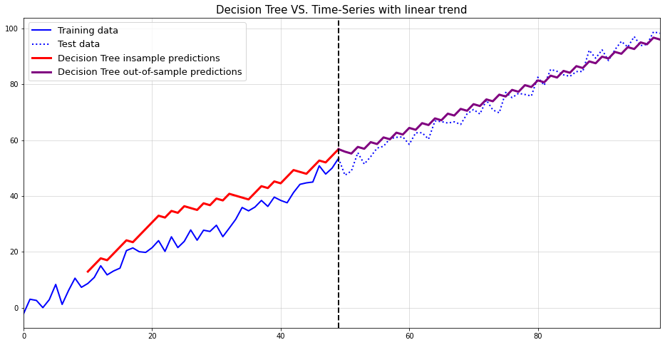
Let us visualize this issue on a quick toy example:

The same issues obviously arise for seasonal patterns as well:

To generalize the above in a single sentence:
Decision Trees fail for out-of-distribution data but in regression against time, every future point in time is out-of-distribution.
Thus, we need to find a different approach.
A far more promising approach is the auto-regressive one. Here, we simply view the future of a random variable as dependent on its past realizations.

While this approach is easier to handle than regression on time, it doesn’t come without a cost:
- The time-series must be observed at equi-distant timestamps: If your time-series is measured at random times, you cannot use this approach without further adjustments.
- The time-series should not contain missing values: For many time-series models, this requirement is not mandatory. Our Decision Tree/Random Forest forecaster, however, will require a fully observed time-series.
As these caveats are common for most popular time-series approaches, they aren’t too much of an issue.
Now, before jumping into an example, we need to take a another look at a previously discussed issue: Tree based models can only predict within the range of training data. This implies that we cannot just fit a Decision Tree or Random Forest to model auto-regressive dependencies.
To exemplify this issue, let’s do another example:

Again, not useful at all. To fix this last issue, we need to first remove the trend. Then we can fit the model, forecast the time-series and ‘re-trend’ the forecast.
For de-trending, we basically have two options:
- Fit a linear trend model — here we regress the time-series against time in a linear regression model. Its predictions are then subtracted from the training data to create a stationary time-series. This removes a constant, deterministic trend.
- Use first-differences — in this approach, we transform the time-series via first order differencing. In addition to the deterministic trend, this approach can also remove stochastic trends.
As most time-series are driven by randomness, the second approach appears more reasonable. Thus, we now aim to forecast the transformed time-series

by an autoregressive model, i.e.

Obviously, differencing and lagging remove some observations from our training data. Some care should be taken to not remove too much information that way. I.e. don’t use too many lagged variables if your dataset is small.
To obtain a forecast for the original time-series we need to retransform the differenced forecast via

and, recursively for further ahead forecasts:

For our running example this finally leads to a reasonable solution:
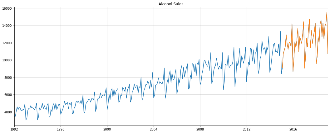
Let us now apply the above approach to a real-world dataset. We use the alcohol sales data from the St. Louis Fed database. For evaluation, we use the last four years as a holdout set:
Since a single Decision Tree would be boring at best and inaccurate at worst, we’ll use a Random Forest instead. Besides the typical performance improvements, Random Forests allow us to generate forecast intervals.
To create Random Forest forecast intervals, we proceed as follows:
- Train an autoregressive Random Forest: This step is equivalent to fitting the Decision Tree as before
- Use a randomly drawn Decision Tree at each forecast step: Instead of just
forest.predict(), we let a randomly drawn, single Decision Tree perform the forecast. By repeating this step multiple times, we create a sample of Decision Tree forecasts. - Calculate quantities of interest from the Decision Tree sample: This could range from median to standard deviation or more complex targets. We are primarily interested in a mean forecast and the 90% predictive interval.
The following Python class does everything we need:
As our data is strictly positive, has a trend and yearly seasonality, we apply the following transformations:
- Logarithm transformation: Our forecasts then need to be re-transformed via an exponential transform. Thus, the exponentiated results will be strictly positive as well
- First differences: As mentioned above, this removes the linear trend in the data.
- Seasonal differences: Seasonal differencing works like first differences with higher lag orders. Also, it allows us to remove both deterministic and stochastic seasonality.
The main challenge with all these transformations is to correctly apply their inverse on our predictions. Luckily, the above model has these steps implemented already.
Using the data and the model, we get the following result for our test period:

This looks quite good. To verify that we were not just lucky, we use a simple benchmark for comparison:

Apparently, the benchmark intervals are much worse than for the Random Forest. The mean forecast starts out reasonably but quickly deteriorates after a few steps.
Let’s compare both mean forecasts in a single chart:

Clearly, the Random Forest is far superior for longer horizon forecasts. In fact, Random Forest has an RMSE of 909.79 while the benchmark’s RMSE is 9745.30.
Hopefully, this article gave you some insights on the do’s and dont’s of forecasting with tree models. While a single Decision Tree might be useful sometimes, Random Forests are usually more performant. That is, unless your dataset is very tiny in which case you could still reduce max_depth of your forest trees.
Obviously, you could add easily add external regressors to either model to improve performance further. As an example, adding monthly indicators to our model might yield more accurate results than right now.
As an alternative to Random Forests, Gradient Boosting could be considered. Nixtla’s mlforecast package has a very powerful implementation — besides all their other great tools for forecasting. Keep in mind however, that we cannot transfer the algorithm for forecast intervals to Gradient Boosting.
On another note, keep in mind that forecasting with advanced machine learning is a double-edged sword. While powerful at the surface, ML for time-series can overfit much quicker than for cross-sectional problems. As long as you properly test your model against some benchmarks, though, they should not be overlooked either.
PS: You can find a full notebook for this article here.
[1] Breiman, Leo. Random forests. Machine learning, 2001, 45.1, p. 5–32.
[2] Breiman, Leo, et al. Classification and regression trees. Routledge, 2017.
[3] Hamilton, James Douglas. Time series analysis. Princeton university press, 2020.
[4] U.S. Census Bureau, Merchant Wholesalers, Except Manufacturers’ Sales Branches and Offices: Nondurable Goods: Beer, Wine, and Distilled Alcoholic Beverages Sales [S4248SM144NCEN], retrieved from FRED, Federal Reserve Bank of St. Louis; https://fred.stlouisfed.org/series/S4248SM144NCEN (CC0: Public Domain)
Random Forests are flexible and powerful when it comes to tabular data. Do they also work for time-series forecasting? Let’s find out.

Today, Deep Learning dominates many areas of modern machine learning. On the other hand, Decision Tree based models still shine particularly for tabular data. If you look up the winning solutions of respective Kaggle challenges, chances are high that a tree model is among them.
A key advantage of tree approaches is that they typically don’t require too much fine-tuning for reasonable results. This is in stark contrast to Deep Learning. Here, different topologies and architectures can result in dramatical differences in model performance.
For time-series forecasting, decision trees are not as straightforward as for tabular data, though:
As you probably know, fitting any decision tree based methods requires both input and output variables. In a univariate time-series problem, however, we usually only have our time-series as a target.
To work around this issue, we need to augment the time-series to become suitable for tree models. Let us discuss two intuitive, yet false approaches and why they fail first. Obviously, the issues generalize to all Decision Tree ensemble methods.
Decision Tree forecasting as regression against time
Probably the most intuitive approach is to consider the observed time-series as a function of time itself, i.e.
With some i.i.d. stochastic additive error term. In an earlier article, I have already made some remarks on why regression against time itself is problematic. For tree based models, there is another problem:
Decision Trees for regression against time cannot extrapolate into the future.
By construction, Decision Tree predictions are averages of subsets of the training dataset. These subsets are formed by splitting the space of input data into axis-parallel hyper rectangles. Then, for each hyper rectangle, we take the average of all observation outputs inside those rectangles as a prediction.
For regression against time, those hyper rectangles are simply splits of time intervals. More exactly, those intervals are mutually exclusive and completely exhaustive.
Predictions are then the arithmetic means of the time-series observations inside those intervals. Mathematically, this roughly translates to
Consider now using this model to predict the time-series at some time in the future. This reduces the above formula to the following:
In words: For any forecast, our model always predicts the average of the final training interval. Which is clearly useless…
Let us visualize this issue on a quick toy example:
The same issues obviously arise for seasonal patterns as well:
To generalize the above in a single sentence:
Decision Trees fail for out-of-distribution data but in regression against time, every future point in time is out-of-distribution.
Thus, we need to find a different approach.
A far more promising approach is the auto-regressive one. Here, we simply view the future of a random variable as dependent on its past realizations.
While this approach is easier to handle than regression on time, it doesn’t come without a cost:
- The time-series must be observed at equi-distant timestamps: If your time-series is measured at random times, you cannot use this approach without further adjustments.
- The time-series should not contain missing values: For many time-series models, this requirement is not mandatory. Our Decision Tree/Random Forest forecaster, however, will require a fully observed time-series.
As these caveats are common for most popular time-series approaches, they aren’t too much of an issue.
Now, before jumping into an example, we need to take a another look at a previously discussed issue: Tree based models can only predict within the range of training data. This implies that we cannot just fit a Decision Tree or Random Forest to model auto-regressive dependencies.
To exemplify this issue, let’s do another example:
Again, not useful at all. To fix this last issue, we need to first remove the trend. Then we can fit the model, forecast the time-series and ‘re-trend’ the forecast.
For de-trending, we basically have two options:
- Fit a linear trend model — here we regress the time-series against time in a linear regression model. Its predictions are then subtracted from the training data to create a stationary time-series. This removes a constant, deterministic trend.
- Use first-differences — in this approach, we transform the time-series via first order differencing. In addition to the deterministic trend, this approach can also remove stochastic trends.
As most time-series are driven by randomness, the second approach appears more reasonable. Thus, we now aim to forecast the transformed time-series
by an autoregressive model, i.e.
Obviously, differencing and lagging remove some observations from our training data. Some care should be taken to not remove too much information that way. I.e. don’t use too many lagged variables if your dataset is small.
To obtain a forecast for the original time-series we need to retransform the differenced forecast via
and, recursively for further ahead forecasts:
For our running example this finally leads to a reasonable solution:
Let us now apply the above approach to a real-world dataset. We use the alcohol sales data from the St. Louis Fed database. For evaluation, we use the last four years as a holdout set:
Since a single Decision Tree would be boring at best and inaccurate at worst, we’ll use a Random Forest instead. Besides the typical performance improvements, Random Forests allow us to generate forecast intervals.
To create Random Forest forecast intervals, we proceed as follows:
- Train an autoregressive Random Forest: This step is equivalent to fitting the Decision Tree as before
- Use a randomly drawn Decision Tree at each forecast step: Instead of just
forest.predict(), we let a randomly drawn, single Decision Tree perform the forecast. By repeating this step multiple times, we create a sample of Decision Tree forecasts. - Calculate quantities of interest from the Decision Tree sample: This could range from median to standard deviation or more complex targets. We are primarily interested in a mean forecast and the 90% predictive interval.
The following Python class does everything we need:
As our data is strictly positive, has a trend and yearly seasonality, we apply the following transformations:
- Logarithm transformation: Our forecasts then need to be re-transformed via an exponential transform. Thus, the exponentiated results will be strictly positive as well
- First differences: As mentioned above, this removes the linear trend in the data.
- Seasonal differences: Seasonal differencing works like first differences with higher lag orders. Also, it allows us to remove both deterministic and stochastic seasonality.
The main challenge with all these transformations is to correctly apply their inverse on our predictions. Luckily, the above model has these steps implemented already.
Using the data and the model, we get the following result for our test period:
This looks quite good. To verify that we were not just lucky, we use a simple benchmark for comparison:
Apparently, the benchmark intervals are much worse than for the Random Forest. The mean forecast starts out reasonably but quickly deteriorates after a few steps.
Let’s compare both mean forecasts in a single chart:
Clearly, the Random Forest is far superior for longer horizon forecasts. In fact, Random Forest has an RMSE of 909.79 while the benchmark’s RMSE is 9745.30.
Hopefully, this article gave you some insights on the do’s and dont’s of forecasting with tree models. While a single Decision Tree might be useful sometimes, Random Forests are usually more performant. That is, unless your dataset is very tiny in which case you could still reduce max_depth of your forest trees.
Obviously, you could add easily add external regressors to either model to improve performance further. As an example, adding monthly indicators to our model might yield more accurate results than right now.
As an alternative to Random Forests, Gradient Boosting could be considered. Nixtla’s mlforecast package has a very powerful implementation — besides all their other great tools for forecasting. Keep in mind however, that we cannot transfer the algorithm for forecast intervals to Gradient Boosting.
On another note, keep in mind that forecasting with advanced machine learning is a double-edged sword. While powerful at the surface, ML for time-series can overfit much quicker than for cross-sectional problems. As long as you properly test your model against some benchmarks, though, they should not be overlooked either.
PS: You can find a full notebook for this article here.
[1] Breiman, Leo. Random forests. Machine learning, 2001, 45.1, p. 5–32.
[2] Breiman, Leo, et al. Classification and regression trees. Routledge, 2017.
[3] Hamilton, James Douglas. Time series analysis. Princeton university press, 2020.
[4] U.S. Census Bureau, Merchant Wholesalers, Except Manufacturers’ Sales Branches and Offices: Nondurable Goods: Beer, Wine, and Distilled Alcoholic Beverages Sales [S4248SM144NCEN], retrieved from FRED, Federal Reserve Bank of St. Louis; https://fred.stlouisfed.org/series/S4248SM144NCEN (CC0: Public Domain)
Denial of responsibility! Techno Blender is an automatic aggregator of the all world’s media. In each content, the hyperlink to the primary source is specified. All trademarks belong to their rightful owners, all materials to their authors. If you are the owner of the content and do not want us to publish your materials, please contact us by email – [email protected]. The content will be deleted within 24 hours.