
Fraud Detection with Generative Adversarial Nets (GANs)
Application of GANs for data augmentation to adjust an imbalanced dataset
“Generative Adversarial Nets” (GANs) demonstrated outstanding performance in generating realistic synthetic data which are indistinguishable from the real data in the past. Unfortunately, GANs caught the public’s attention because of its unethical applications, deepfakes (Knight, 2018).
This article illustrates a case with a good motive in the application of GANs in the context of fraud detection.
Fraud detection is an application of binary classification prediction. Fraud cases, which account for only a small fraction of the transaction universe, constitute a minority class that makes the dataset highly imbalanced. In general, the resulting model tends to be biased towards the majority class and tends to underfit to the minority class. Thus, the less balanced the dataset, the poorer the performance of the classification predictor would be.
My motive here is to use GANs as a data augmentation tool in an attempt to address this classical problem of fraud detection associated with the imbalanced dataset. More specifically, GANs can generate realistic synthetic data of the minority fraud class and transform the imbalanced dataset perfectly balanced.
And, I am hoping that this sophisticated algorithm could materially contribute to the performance of fraud detection. In other words, my initial expectation is: the better sophisticated algorithm, the better performance.
A relevant question is if the use of GANs will guarantee a promising improvement in the performance of fraud detection and satisfy my motive. Let’s see.
Introduction
In principle, fraud detection is an application of binary classification algorithm: to classify each transaction whether it is a fraud case or not.
Fraud cases account for only a small fraction of the transaction universe. In general, fraud cases constitute the minority class, thus, make the dataset highly imbalanced.
The fewer fraud cases, the more sound the transaction system would be.
Very simple and intuitive.
Paradoxically, that sound condition was one of the primary reasons that made fraud detection challenging in the past, if not impossible. It is simply because it was difficult for a classification algorithm to learn the probability distribution of the minority class of fraud.
In general, the more balanced the dataset, the better the performance of the classification predictor. In other words, the less balanced (or the more imbalanced) the dataset, the poorer the performance of classifier.
This paints the classical problem of fraud detection: a binary classification application with highly imbalanced dataset.
In this setting, we can use Generative Adversarial Nets (GANs) as a data augmentation tool to generate realistic synthetic data of the minority fraud class to transform the entire dataset more balanced in an attempt to improve the performance of the classifier model of fraud detection.
This article is divided into the following sections:
- Section 1: Algorithm Overview: Bi-level Optimization Architecture of GANs
- Section 2: Fraud Dataset
- Section 3: Python Code breakdown of GANs for data augmentation
- Section 4: Fraud Detection Overview (Benchmark Scenario vs GANs Scenario)
- Section 5: Conclusion
Overall, I will primarily focus on the topic of GANs (both the algorithm and the code). For the remaining topics of the model development other than GANs, such as data preprocessing and classifier algorithm, I will only outline the process and refrain from going into their details. In this context, this article assumes that the readers have a basic knowledge about the binary classifier algorithm (especially, Ensemble Classifier that I selected for fraud detection) as well as general understanding of data cleaning and preprocessing.
For the detailed code, the readers are welcome to access the following link: https://github.com/deeporigami/Portfolio/blob/6538fcaad1bf58c5f63d6320ca477fa867edb1df/GAN_FraudDetection_Medium_2.ipynb
Section 1: Algorithm Overview: Bi-level Optimization Architecture of GANs
GANs is a special type of generative algorithm. As its name suggests, Generative Adversarial Nets (GANs) is composed of two neural networks: the generative network (the generator) and the adversarial network (the discriminator). GANs pits these two agents against each other to engage in a competition, where the generator attempts to generate realistic synthetic data and the discriminator to distinguish the synthetic data from the real data.
The original GANs was introduced in a seminal paper: “Generative Adversarial Nets” (Goodfellow, et al., Generative Adversarial Nets, 2014). The co-authors of the original GANs portrayed GANs with a counterfeiter-police analogy: an iterative game, where the generator acts as a counterfeiter and the discriminator plays the role of the police to detect the counterfeit that the generator forged.
The original GANs was innovative in a sense that it addressed and overcame conventional difficulties in training deep generative algorithm in the past. And as its core, it was designed with bi-level optimization framework with an equilibrium seeking objective setting (vs maximum likelihood oriented objective setting).
Ever since, many variant architectures of GANs have been explored. As a precaution, this article refers solely to the prototype architecture of the original GANs.
Generator and Discriminator
Repeatedly, in the architecture of GANs, the two neural networks — the generator and the discriminator — compete against each other. In this context, the competition takes place through the iteration of forward propagation and backward propagation (according to the general framework of neural networks).
On one hand, it is straight-forward that the discriminator is a binary classifier by design: it classifies whether each sample is real (label: 1) or fake/synthetic (label:0). And the discriminator is fed with both the real samples and the synthetic samples during the forward propagation. Then, during the backpropagation, it learns to detect the synthetic data from the mixed data feed.
On the other hand, the generator is a noise distribution by design. The generator is fed with the real samples during the forward propagation. Then, during the backward propagation, the generator learns the probability distribution of the real data in order to better simulate its synthetic samples.
And these two agents are trained alternately via “bi-level optimization” framework.
Bi-level Training Mechanism (bi-level optimization method)
In the original GAN paper, in order to train these two agents that pursue their diametrically opposite objectives, the co-authors designed a “bi-level optimization (training)” architecture, in which one internal training block (training of the discriminator) is nested within another high-level training block (training of the generator).
The image below illustrates the structure of “bi-level optimization” in the nested training loops. The discriminator is trained within the nested inner loop, while the generator is trained in the main loop at the higher level.
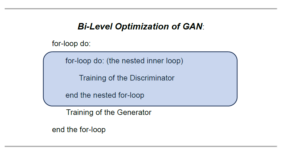
And GANs trains these two agents alternately in this bi-level training architecture (Goodfellow, et al., Generative Adversarial Nets, 2014, p. 3). In other words, while training one agent during the alternation, we need to freeze the learning process of the other agent (Goodfellow I. , 2015, p. 3).
Mini-Max Optimization Objective
In addition to the “bi-level optimization” mechanism which enables the alternate training of these two agents, another unique feature that differentiates GANs from the conventional prototype of neural network is its mini-max optimization objective. Simply put, in contrast to the conventional maximum seeking approach (such as maximum-likelihood) , GANs pursues an equilibrium-seeking optimization objective.
What is an equilibrium-seeking optimization objective?
Let’s break it down.
GANs’ two agents have two diametrically opposite objectives. While the discriminator, as a binary classifier, aims at maximizing the probability of correctly classifying the mixture of the real samples and the synthetic samples, the generator’s objective is to minimize the probability that the discriminator correctly classifies the synthetic data: simply because the generator needs to fool the discriminator.
In this context, the co-authors of the original GANs called the overall objective a “minimax game”. (Goodfellow, et al., 2014, p. 3)
Overall, the ultimate mini-max optimization objective of GANs is not to search for the global maximum/minimum of either of these objective functions. Instead, it is set to seek an equilibrium point which can be interpreted as:
- “a saddle point that is a local maximum for the classifier and a local minimum for the generator” (Goodfellow I. , 2015, p. 2)
- where neither of agents can improve their performance any longer.
- where the synthetic data that the generator learned to create has become realistic enough to fool the discriminator.
And the equilibrium point could be conceptually represented by the probability of random guessing, 0.5 (50%), for the discriminator: D(z) => 0.5 .
Let’s transcribe the conceptual framework of GANs’ minimax optimization in terms of their objective functions.
The objective of the discriminator is to maximize the objective function in the following image:

In order to resolve a potential saturation issue, they converted the second term of the original log-likelihood objective function for the generator as follows and recommended to maximize the converted version as the generator’s objective:

Overall, the architecture of GANs’ “bi-level optimization” can be translated in to the following algorithm.

For more details about the algorithmic design of GANs, please read another article of mine: Mini-Max Optimization Design of Generative Adversarial Nets .
Now, let’s move on to the actual coding with a dataset.
In order to highlight GANs algorithm, I will primarily focus on the code of GANs here and only outline the rest of the process.
Section 2: Fraud Dataset
For fraud detection, I selected the following dataset of credit card transactions from Kaggle: https://www.kaggle.com/datasets/mlg-ulb/creditcardfraud
Data License: Database Contents License (DbCL) v1.0
Here is a summary of the dataset.
The dataset contains 284,807 transactions. In the dataset, we have only 492 fraud cases (including 29 duplicated cases).
Since the fraud class accounts for only 0.172% of all transactions, it constitutes an extremely small minority class. This dataset is an appropriate one for illustrating the classical problem of fraud detection associated with the imbalanced dataset.
It has the following 30 features:
- V1, V2, … V28: 28 principal components obtained by PCA. The source of the data is not disclosed for the privacy protection purpose.
- ‘Time’: the seconds elapsed between each transaction and the first transaction of the dataset.
- ‘Amount’: the amount of the transaction.
The label is set as ‘Class’.
- ‘Class’: 1 in case of fraud; and 0 otherwise.
Data Preprocessing: Feature Selection
Since the dataset has already been pretty much, if not perfectly, cleaned, I only had to do few things for the data cleaning: elimination of duplicated data and removal of outliers.
Thereafter, given 30 features in the dataset, I decided to run the feature selection to reduce the number of the features by eliminating less important features before the training process. I selected the built-in feature importance score of the scikit-learn Random Forest Classifier to estimate the scores of all the 30 features.
The following chart displays the summary of the result. If interested in the detailed process, please visit my code listed above.
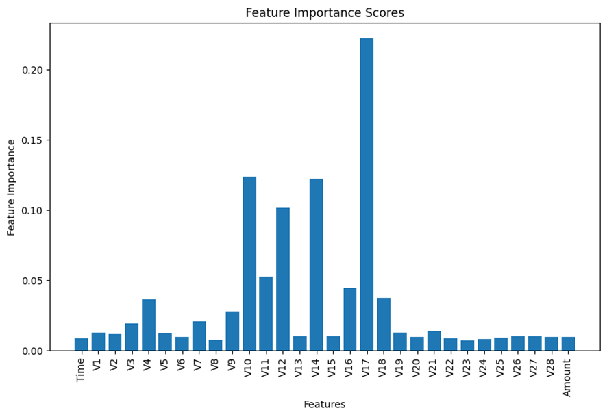
Based on the results displayed in the bar chart above, I made my subjective judgement to select the top 6 features for the analysis and remove all the remaining insignificant features from the model building process.
Here is the selected top 6 important features.
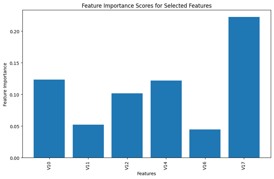
For the model building purpose going forward, I focused on these 6 selected features. After the data preprocessing, we have the working dataframe, df, of the following shape:
- df.shape = (282513, 7)
Hopefully, the feature selection would reduce the complexity of the resulting model and stabilize its performance, while retaining critical information for optimizing a binary classifier.
Scenario 3: Code breakdown of GANs for data augmentation
Finally, it’s time for us to use GANs for data augmentation.
So how many synthetic data do we need to create?
First of all, our interest for the data augmentation is only for the model training. Since the test dataset is out-of-sample data, we want to preserve the original form of the test dataset. Secondly, because our intention is to transform the imbalanced dataset perfectly, we do not want to augment the majority class of non-fraud cases.
Simply put, we want to augment only the train dataset of the minority fraud class, nothing else.
Now, let’s split the working dataframe into the train dataset and the test dataset in 80/20 ratio, using a stratified data split method.
# Separate features and target variable
X = df.drop('Class', axis=1)
y = df['Class']

# Splitting data into train and test sets
X_train, X_test, y_train, y_test = train_test_split(X, y, test_size=0.2, random_state=42, stratify=y)

# Combine the features and the label for the train dataset
train_df = pd.concat([X_train, y_train], axis=1)
As a result, the shape of the train dataset is as follows:
- train_df.shape = (226010, 7)
Let’s see the composition (the fraud cases and the non-fraud cases) of the train dataset.
# Load the dataset (fraud and non-fraud data)
fraud_data = train_df[train_df['Class'] == 1].drop('Class', axis=1).values
non_fraud_data = train_df[train_df['Class'] == 0].drop('Class', axis=1).values

# Calculate the number of synthetic fraud samples to generate
num_real_fraud = len(fraud_data)
num_synthetic_samples = len(non_fraud_data) - num_real_fraud
print("# of non-fraud: ", len(non_fraud_data))
print("# of Real Fraud:", num_real_fraud)
print("# of Synthetic Fraud required:", num_synthetic_samples)

# of non-fraud:  225632
# of Real Fraud: 378
# of Synthetic Fraud required: 225254
This tells us that the train dataset (226,010) is comprised of 225,632 non-fraud data and 378 fraud data. In other words, the difference between them is 225,254. This number is the number of the synthetic fraud data (num_synthetic_samples) that we need to augment in order to perfectly match the numbers of these two classes within the train dataset: as a reminder, we do preserve the original test dataset.
Next, let’s code GANs.
First, let’s create custom functions to determine the two agents: the discriminator and the generator.
For the generator, I create a noise distribution function, build_generator(), which requires two parameters: latent_dim (the dimension of the noise) as the shape of its input; and the shape of its output, output_dim, which corresponds to the number of the features.
# Define the generator network
def build_generator(latent_dim, output_dim):
    model = Sequential()
    model.add(Dense(64, input_shape=(latent_dim,)))
    model.add(Dense(128, activation='sigmoid'))
    model.add(Dense(output_dim, activation='sigmoid'))
    return model
For the discriminator, I create a custom function build_discriminator() that takes input_dim, which corresponds to the number of the features.
# Define the discriminator network
def build_discriminator(input_dim):
    model = Sequential()
    model.add(Input(input_dim))
    model.add(Dense(128, activation='sigmoid'))
    model.add(Dense(1, activation='sigmoid'))
    return model
Then, we can call these function to create the generator and the discriminator. Here, for the generator I arbitrarily set latent_dim to be 32: you can try other value here, if you like.
# Dimensionality of the input noise for the generator
latent_dim = 32

# Build generator and discriminator models
generator = build_generator(latent_dim, fraud_data.shape[1])
discriminator = build_discriminator(fraud_data.shape[1])
At this stage, we need to compile the discriminator, which is going to be nested in the main (higher) optimization loop later. And we can compile the discriminator with the following argument setting.
- the loss function of the discriminator: the generic cross-entropy loss function for a binary classifier
- the evaluation metrics: precision and recall.
# Compile the discriminator model
from keras.metrics import Precision, Recall
discriminator.compile(optimizer=Adam(learning_rate=0.0002, beta_1=0.5), loss='binary_crossentropy',  metrics=[Precision(), Recall()])
For the generator, we will compile it when we construct the main (upper) optimization loop.
At this stage, we can define the custom objective function for the generator as follows. Remember, the recommended objective was to maximize the following formula:
def generator_loss_log_d(y_true, y_pred):
    return - K.mean(K.log(y_pred + K.epsilon()))
Above, the negative sign is required, since the loss function by default is designed to be minimized.
Then, we can construct the main (upper) loop, build_GANs(generator, discriminator), of the bi-level optimization architecture. In this main loop, we compile the generator implicitly. In this context, we need to use the custom objective function of the generator, generator_loss_log_d, when we compile the main loop.
As aforementioned, we need to freeze the discriminator when we train the generator.
# Build and compile the GANs upper optimization loop combining generator and discriminator
def build_gan(generator, discriminator):
    discriminator.trainable = False
    model = Sequential()
    model.add(generator)
    model.add(discriminator)
    model.compile(optimizer=Adam(learning_rate=0.0002, beta_1=0.5), loss=generator_loss_log_d)

    return model

# Call the upper loop function
gan = build_gan(generator, discriminator)
At the last line above, gan calls build_gan() in order to implement the batch training below, using Keras’ model.train_on_batch() method.
As a reminder, while we train the discriminator, we need to freeze the training of the generator; and while we train the generator, we need to freeze the training of the discriminator.
Here is the batch training code incorporating the alternating training process of these two agents under the bi-level optimization framework.
# Set hyperparameters
epochs = 10000
batch_size = 32

# Training loop for the GANs
for epoch in range(epochs):
    # Train discriminator (freeze generator)
    discriminator.trainable = True
    generator.trainable = False

    # Random sampling from the real fraud data
    real_fraud_samples = fraud_data[np.random.randint(0, num_real_fraud, batch_size)]

    # Generate fake fraud samples using the generator
    noise = np.random.normal(0, 1, size=(batch_size, latent_dim))
    fake_fraud_samples = generator.predict(noise)

    # Create labels for real and fake fraud samples
    real_labels = np.ones((batch_size, 1))
    fake_labels = np.zeros((batch_size, 1))

    # Train the discriminator on real and fake fraud samples
    d_loss_real = discriminator.train_on_batch(real_fraud_samples, real_labels)
    d_loss_fake = discriminator.train_on_batch(fake_fraud_samples, fake_labels)
    d_loss = 0.5 * np.add(d_loss_real, d_loss_fake)

    # Train generator (freeze discriminator)
    discriminator.trainable = False
    generator.trainable = True

    # Generate synthetic fraud samples and create labels for training the generator
    noise = np.random.normal(0, 1, size=(batch_size, latent_dim))
    valid_labels = np.ones((batch_size, 1))

    # Train the generator to generate samples that "fool" the discriminator
    g_loss = gan.train_on_batch(noise, valid_labels)

    # Print the progress
    if epoch % 100 == 0:
        print(f"Epoch: {epoch} - D Loss: {d_loss} - G Loss: {g_loss}")
Here, I have a quick question for you.
Below we have an excerpt associated with the generator training from the code above.
Can you explain what this code is doing?
# Generate synthetic fraud samples and create labels for training the generator
    noise = np.random.normal(0, 1, size=(batch_size, latent_dim))
    valid_labels = np.ones((batch_size, 1))
In the first line, noise generates the synthetic data. In the second line, valid_labels assigns the label of the synthetic data.
Why do we need to label it with 1, which is supposed to be the label for the real data? Didn’t you find the code counter-intuitive?
Ladies and gentlemen, welcome to the world of counterfeiters.
This is the labeling magic that trains the generator to create samples that can fool the discriminator.
Now, let’s use the trained generator to create the synthetic data for the minority fraud class.
# After training, use the generator to create synthetic fraud data
noise = np.random.normal(0, 1, size=(num_synthetic_samples, latent_dim))
synthetic_fraud_data = generator.predict(noise)

# Convert the result to a Pandas DataFrame format
fake_df = pd.DataFrame(synthetic_fraud_data, columns=features.to_list())
Finally, the synthetic data is created.
In the next section, we can combine this synthetic fraud data with the original train dataset to make the entire train dataset perfectly balanced. I hope that the perfectly balanced training dataset would improve the performance of the fraud detection classification model.
Section 4: Fraud Detection Overview (with and without GANs data augmentation)
Repeatedly, the use of GANs in this project is exclusively for data augmentation, but not for classification.
First of all, we would need the benchmark model as the basis of the comparison in order for us to evaluate the improvement made by the GANs based data augmentation on the performance of the fraud detection model.
As a binary classifier algorithm, I selected Ensemble Method for building the fraud detection model. As the benchmark scenario, I developed a fraud detection model only with the original imbalanced dataset: thus, without data augmentation. Then, for the second scenario with data augmentation by GANs, I can train the same algorithm with the perfectly balanced train dataset, which contains the synthetic fraud data created by GANs.
- Benchmark Scenario: Ensemble Classifier without data augmentation
- GANs Scenario: Ensemble Classifier with data augmentation by GANs
Benchmark Scenario: Ensemble without data augmentation
Next, let’s define the benchmark scenario (without data augmentation). I decided to select Ensemble Classifier: voting method as the meta learner with the following 3 base learners.
- Gradient Boosting
- Decision Tree
- Random Forest
Since the original dataset is highly imbalanced, rather than accuracy I shall select evaluation metrics from the following 3 options: precision, recall, and F1-Score.
The following custom function, ensemble_training(X_train, y_train), defines the training and validation process.
def ensemble_training(X_train, y_train):
  # Initialize base learners
  gradient_boosting = GradientBoostingClassifier(random_state=42)
  decision_tree = DecisionTreeClassifier(random_state=42)
  random_forest = RandomForestClassifier(random_state=42)
  # Define the base models
  base_models = {
    'RandomForest': random_forest,
    'DecisionTree': decision_tree,
    'GradientBoosting': gradient_boosting
  }
  # Initialize the meta learner
  meta_learner = VotingClassifier(estimators=[(name, model) for name, model in base_models.items()], voting='soft')
  # Lists to store training and validation metrics
  train_f1_scores = []
  val_f1_scores = []
  # Splitting the train set further into training and validation sets
  X_train, X_val, y_train, y_val = train_test_split(X_train, y_train, test_size=0.25, random_state=42, stratify=y_train)
  # Training and validation
  for model_name, model in base_models.items():
    model.fit(X_train, y_train)
    # Training metrics
    train_predictions = model.predict(X_train)
    train_f1 = f1_score(y_train, train_predictions)
    train_f1_scores.append(train_f1)
    # Validation metrics using the validation set
    val_predictions = model.predict(X_val)
    val_f1 = f1_score(y_val, val_predictions)
    val_f1_scores.append(val_f1)
  # Training the meta learner on the entire training set
  meta_learner.fit(X_train, y_train)
return meta_learner, train_f1_scores, val_f1_scores, base_models
The next function block, ensemble_evaluations(meta_learner, X_train, y_train, X_test, y_test), calculates the performance evaluation metrics at the meta learner level.
def ensemble_evaluations(meta_learner,X_train, y_train, X_test, y_test):
# Metrics for the ensemble model on both traininGANsd test datasets
  ensemble_train_predictions = meta_learner.predict(X_train)
  ensemble_test_predictions = meta_learner.predict(X_test)
  # Calculating metrics for the ensemble model
  ensemble_train_f1 = f1_score(y_train, ensemble_train_predictions)
  ensemble_test_f1 = f1_score(y_test, ensemble_test_predictions)
  # Calculate precision and recall for both training and test datasets
  precision_train = precision_score(y_train, ensemble_train_predictions)
  recall_train = recall_score(y_train, ensemble_train_predictions)
  precision_test = precision_score(y_test, ensemble_test_predictions)
  recall_test = recall_score(y_test, ensemble_test_predictions)
  # Output precision, recall, and f1 score for both training and test datasets
  print("Ensemble Model Metrics:")
  print(f"Training Precision: {precision_train:.4f}, Recall: {recall_train:.4f}, F1-score: {ensemble_train_f1:.4f}")
  print(f"Test Precision: {precision_test:.4f}, Recall: {recall_test:.4f}, F1-score: {ensemble_test_f1:.4f}")
return ensemble_train_predictions, ensemble_test_predictions, ensemble_train_f1, ensemble_test_f1, precision_train, recall_train, precision_test, recall_test
Below, let’s look at the performance of the benchmark Ensemble Classifier.
Training Precision: 0.9811, Recall: 0.9603, F1-score: 0.9706
Test Precision: 0.9351, Recall: 0.7579, F1-score: 0.8372
At the meta-learner level, the benchmark model generated F1-Score at a reasonable level of 0.8372.
Next, let’s move on to the scenario with data augmentation using GANs . We want to see if the performance of the scenario with GAN can outperform the benchmark scenario.
GANs Scenario: Fraud Detection with data augmentation by GANs
Finally, we have constructed a perfectly balanced dataset by combining the original imbalanced train dataset (both non-fraud and fraud cases), train_df, and the synthetic fraud dataset generated by GANs, fake_df. Here, we will preserve the test dataset as original by not involving it in this process.
wdf = pd.concat([train_df, fake_df], axis=0)
We will train the same ensemble method with the mixed balanced dataset to see if it will outperform the benchmark model.
Now, we need to split the mixed balanced dataset into the features and the label.
X_mixed = wdf[wdf.columns.drop("Class")]
y_mixed = wdf["Class"]
Remember, when I ran the benchmark scenario earlier, I already defined the necessary custom function blocks to train and evaluate the ensemble classifier. I can use those custom functions here as well to train the same Ensemble algorithm with the combined balanced data.
We can pass the features and the label (X_mixed, y_mixed) into the custom Ensemble Classifier function ensemble_training().
meta_learner_GANs, train_f1_scores_GANs, val_f1_scores_GANs, base_models_GANs=ensemble_training(X_mixed, y_mixed)
Finally, we can evaluate the model with the test dataset.
ensemble_evaluations(meta_learner_GANs, X_mixed, y_mixed, X_test, y_test)
Here is the result.
Ensemble Model Metrics:
Training Precision: 1.0000, Recall: 0.9999, F1-score: 0.9999
Test Precision: 0.9714, Recall: 0.7158, F1-score: 0.8242
Conclusion
Finally, we can assess whether the data augmentation by GANs improved the performance of the classifier, as I expected.
Let’s compare the evaluation metrics between the benchmark scenario and GANs scenario.
Here is the result from the benchmark scenario.
# The Benchmark Scenrio without data augmentation by GANs
Training Precision: 0.9811, Recall: 0.9603, F1-score: 0.9706
Test Precision: 0.9351, Recall: 0.7579, F1-score: 0.8372
Here is the result from GANs scenario.
Training Precision: 1.0000, Recall: 0.9999, F1-score: 0.9999
Test Precision: 0.9714, Recall: 0.7158, F1-score: 0.8242
When we review the evaluation results on the training dataset, clearly GANs scenario outperformed the benchmark scenario over all the three evaluation metrics.
Nevertheless, when we focus on the results on the out-of-sample test data, GANs scenario outperformed the benchmark scenario only for precision (Benchmark: 0.935 vs GANs Scenario: 0.9714): it failed do so for recall and F1-Score (Benchmark: 0.7579; 0.8372 vs GANs Scenario: 0.7158; 0.8242).
- A higher precision means that the model’s prediction of fraud cases did include less proportion of non-fraud cases than the benchmark scenario.
- A lower recall means that the model failed to detect certain varieties of the actual fraud cases.
These two comparisons indicate: while the data augmentation by GANs was successful in simulating the realistic fraud data within the training dataset, it has failed to capture the diversity of the actual fraud cases included in the out-of-sample test dataset.
GANs was too good in simulating the particular probability distribution of the train data. Ironically, as a result, the use of GANs as the data augmentation tool, accounting for overfitting to the train data, resulted in a poor generalization of the resulting fraud detection (classification) model.
Paradoxically, this particular example made a counter-intuitive case that a better sophisticated algorithm might not necessarily guarantee a better performance when compared with simpler conventional algorithms.
In addition, we could also take into account of another unintended consequence, wasteful carbon footprint: adding energy demanding algorithms into your model development could increase the carbon footprint in the use of the machine learning in our daily life. This case could illustrate an example of an unnecessarily wasteful case which wasted energy unnecessarily without delivering a better performance.
Here I leave you some links regarding energy consumption of machine learning.
- https://spectrum.ieee.org/ai-energy-consumption
- https://www.cell.com/joule/fulltext/S2542-4351(23)00365-3?_returnURL=https%3A%2F%2Flinkinghub.elsevier.com%2Fretrieve%2Fpii%2FS2542435123003653%3Fshowall%3Dtrue
Today, we have many variants of GANs. In the future article, I would like to explore other variants of GANs to see if any variant can capture a wider diversity of the original samples so that it can improve the performance of a fraud detector.
Thanks for reading.
Michio Suginoo
REFERENCE
- Borji, A. (2018, 10 24). Pros and Cons of GAN Evaluation Measures. Retrieved from ArXvi: https://arxiv.org/abs/1802.03446
- Goodfellow, I. (2015, 5 21). On distinguishability criteria for estimating generative models. Retrieved from ArXiv: https://arxiv.org/abs/1412.6515
- Goodfellow, I. J., Pouget-Abadie, J., Mirza, M., Xu, B., Warde-Farley, D., Ozairy, S., . . . Bengioz, Y. (2014, 6 10). Generative Adversarial Nets. Retrieved from arXiv: https://arxiv.org/abs/1406.2661
- Goodfellow, I. J., Pouget-Abadie, J., Mirza, M., Xu, B., Warde-Farley, D., Ozairy, S., . . . Bengioz, Y. (2014, 6 10). Generative Adversarial Networks. Retrieved from arXiv: https://arxiv.org/abs/1406.2661
- Knight, W. (2018, 8 17). Fake America great again. Retrieved from MIT Technology Review: https://www.technologyreview.com/2018/08/17/240305/fake-america-great-again/
- Suginoo, M. (2024, 1 13). Mini-Max Optimization Design of Generative Adversarial Networks (GAN). Retrieved from Towards Data Science: https://towardsdatascience.com/mini-max-optimization-design-of-generative-adversarial-networks-gan-dc1b9ea44a02
Fraud Detection with Generative Adversarial Nets (GANs) was originally published in Towards Data Science on Medium, where people are continuing the conversation by highlighting and responding to this story.
Application of GANs for data augmentation to adjust an imbalanced dataset

“Generative Adversarial Nets” (GANs) demonstrated outstanding performance in generating realistic synthetic data which are indistinguishable from the real data in the past. Unfortunately, GANs caught the public’s attention because of its unethical applications, deepfakes (Knight, 2018).
This article illustrates a case with a good motive in the application of GANs in the context of fraud detection.
Fraud detection is an application of binary classification prediction. Fraud cases, which account for only a small fraction of the transaction universe, constitute a minority class that makes the dataset highly imbalanced. In general, the resulting model tends to be biased towards the majority class and tends to underfit to the minority class. Thus, the less balanced the dataset, the poorer the performance of the classification predictor would be.
My motive here is to use GANs as a data augmentation tool in an attempt to address this classical problem of fraud detection associated with the imbalanced dataset. More specifically, GANs can generate realistic synthetic data of the minority fraud class and transform the imbalanced dataset perfectly balanced.
And, I am hoping that this sophisticated algorithm could materially contribute to the performance of fraud detection. In other words, my initial expectation is: the better sophisticated algorithm, the better performance.
A relevant question is if the use of GANs will guarantee a promising improvement in the performance of fraud detection and satisfy my motive. Let’s see.
Introduction
In principle, fraud detection is an application of binary classification algorithm: to classify each transaction whether it is a fraud case or not.
Fraud cases account for only a small fraction of the transaction universe. In general, fraud cases constitute the minority class, thus, make the dataset highly imbalanced.
The fewer fraud cases, the more sound the transaction system would be.
Very simple and intuitive.
Paradoxically, that sound condition was one of the primary reasons that made fraud detection challenging in the past, if not impossible. It is simply because it was difficult for a classification algorithm to learn the probability distribution of the minority class of fraud.
In general, the more balanced the dataset, the better the performance of the classification predictor. In other words, the less balanced (or the more imbalanced) the dataset, the poorer the performance of classifier.
This paints the classical problem of fraud detection: a binary classification application with highly imbalanced dataset.
In this setting, we can use Generative Adversarial Nets (GANs) as a data augmentation tool to generate realistic synthetic data of the minority fraud class to transform the entire dataset more balanced in an attempt to improve the performance of the classifier model of fraud detection.
This article is divided into the following sections:
- Section 1: Algorithm Overview: Bi-level Optimization Architecture of GANs
- Section 2: Fraud Dataset
- Section 3: Python Code breakdown of GANs for data augmentation
- Section 4: Fraud Detection Overview (Benchmark Scenario vs GANs Scenario)
- Section 5: Conclusion
Overall, I will primarily focus on the topic of GANs (both the algorithm and the code). For the remaining topics of the model development other than GANs, such as data preprocessing and classifier algorithm, I will only outline the process and refrain from going into their details. In this context, this article assumes that the readers have a basic knowledge about the binary classifier algorithm (especially, Ensemble Classifier that I selected for fraud detection) as well as general understanding of data cleaning and preprocessing.
For the detailed code, the readers are welcome to access the following link: https://github.com/deeporigami/Portfolio/blob/6538fcaad1bf58c5f63d6320ca477fa867edb1df/GAN_FraudDetection_Medium_2.ipynb
Section 1: Algorithm Overview: Bi-level Optimization Architecture of GANs
GANs is a special type of generative algorithm. As its name suggests, Generative Adversarial Nets (GANs) is composed of two neural networks: the generative network (the generator) and the adversarial network (the discriminator). GANs pits these two agents against each other to engage in a competition, where the generator attempts to generate realistic synthetic data and the discriminator to distinguish the synthetic data from the real data.
The original GANs was introduced in a seminal paper: “Generative Adversarial Nets” (Goodfellow, et al., Generative Adversarial Nets, 2014). The co-authors of the original GANs portrayed GANs with a counterfeiter-police analogy: an iterative game, where the generator acts as a counterfeiter and the discriminator plays the role of the police to detect the counterfeit that the generator forged.
The original GANs was innovative in a sense that it addressed and overcame conventional difficulties in training deep generative algorithm in the past. And as its core, it was designed with bi-level optimization framework with an equilibrium seeking objective setting (vs maximum likelihood oriented objective setting).
Ever since, many variant architectures of GANs have been explored. As a precaution, this article refers solely to the prototype architecture of the original GANs.
Generator and Discriminator
Repeatedly, in the architecture of GANs, the two neural networks — the generator and the discriminator — compete against each other. In this context, the competition takes place through the iteration of forward propagation and backward propagation (according to the general framework of neural networks).
On one hand, it is straight-forward that the discriminator is a binary classifier by design: it classifies whether each sample is real (label: 1) or fake/synthetic (label:0). And the discriminator is fed with both the real samples and the synthetic samples during the forward propagation. Then, during the backpropagation, it learns to detect the synthetic data from the mixed data feed.
On the other hand, the generator is a noise distribution by design. The generator is fed with the real samples during the forward propagation. Then, during the backward propagation, the generator learns the probability distribution of the real data in order to better simulate its synthetic samples.
And these two agents are trained alternately via “bi-level optimization” framework.
Bi-level Training Mechanism (bi-level optimization method)
In the original GAN paper, in order to train these two agents that pursue their diametrically opposite objectives, the co-authors designed a “bi-level optimization (training)” architecture, in which one internal training block (training of the discriminator) is nested within another high-level training block (training of the generator).
The image below illustrates the structure of “bi-level optimization” in the nested training loops. The discriminator is trained within the nested inner loop, while the generator is trained in the main loop at the higher level.
And GANs trains these two agents alternately in this bi-level training architecture (Goodfellow, et al., Generative Adversarial Nets, 2014, p. 3). In other words, while training one agent during the alternation, we need to freeze the learning process of the other agent (Goodfellow I. , 2015, p. 3).
Mini-Max Optimization Objective
In addition to the “bi-level optimization” mechanism which enables the alternate training of these two agents, another unique feature that differentiates GANs from the conventional prototype of neural network is its mini-max optimization objective. Simply put, in contrast to the conventional maximum seeking approach (such as maximum-likelihood) , GANs pursues an equilibrium-seeking optimization objective.
What is an equilibrium-seeking optimization objective?
Let’s break it down.
GANs’ two agents have two diametrically opposite objectives. While the discriminator, as a binary classifier, aims at maximizing the probability of correctly classifying the mixture of the real samples and the synthetic samples, the generator’s objective is to minimize the probability that the discriminator correctly classifies the synthetic data: simply because the generator needs to fool the discriminator.
In this context, the co-authors of the original GANs called the overall objective a “minimax game”. (Goodfellow, et al., 2014, p. 3)
Overall, the ultimate mini-max optimization objective of GANs is not to search for the global maximum/minimum of either of these objective functions. Instead, it is set to seek an equilibrium point which can be interpreted as:
- “a saddle point that is a local maximum for the classifier and a local minimum for the generator” (Goodfellow I. , 2015, p. 2)
- where neither of agents can improve their performance any longer.
- where the synthetic data that the generator learned to create has become realistic enough to fool the discriminator.
And the equilibrium point could be conceptually represented by the probability of random guessing, 0.5 (50%), for the discriminator: D(z) => 0.5 .
Let’s transcribe the conceptual framework of GANs’ minimax optimization in terms of their objective functions.
The objective of the discriminator is to maximize the objective function in the following image:
In order to resolve a potential saturation issue, they converted the second term of the original log-likelihood objective function for the generator as follows and recommended to maximize the converted version as the generator’s objective:
Overall, the architecture of GANs’ “bi-level optimization” can be translated in to the following algorithm.
For more details about the algorithmic design of GANs, please read another article of mine: Mini-Max Optimization Design of Generative Adversarial Nets .
Now, let’s move on to the actual coding with a dataset.
In order to highlight GANs algorithm, I will primarily focus on the code of GANs here and only outline the rest of the process.
Section 2: Fraud Dataset
For fraud detection, I selected the following dataset of credit card transactions from Kaggle: https://www.kaggle.com/datasets/mlg-ulb/creditcardfraud
Data License: Database Contents License (DbCL) v1.0
Here is a summary of the dataset.
The dataset contains 284,807 transactions. In the dataset, we have only 492 fraud cases (including 29 duplicated cases).
Since the fraud class accounts for only 0.172% of all transactions, it constitutes an extremely small minority class. This dataset is an appropriate one for illustrating the classical problem of fraud detection associated with the imbalanced dataset.
It has the following 30 features:
- V1, V2, … V28: 28 principal components obtained by PCA. The source of the data is not disclosed for the privacy protection purpose.
- ‘Time’: the seconds elapsed between each transaction and the first transaction of the dataset.
- ‘Amount’: the amount of the transaction.
The label is set as ‘Class’.
- ‘Class’: 1 in case of fraud; and 0 otherwise.
Data Preprocessing: Feature Selection
Since the dataset has already been pretty much, if not perfectly, cleaned, I only had to do few things for the data cleaning: elimination of duplicated data and removal of outliers.
Thereafter, given 30 features in the dataset, I decided to run the feature selection to reduce the number of the features by eliminating less important features before the training process. I selected the built-in feature importance score of the scikit-learn Random Forest Classifier to estimate the scores of all the 30 features.
The following chart displays the summary of the result. If interested in the detailed process, please visit my code listed above.
Based on the results displayed in the bar chart above, I made my subjective judgement to select the top 6 features for the analysis and remove all the remaining insignificant features from the model building process.
Here is the selected top 6 important features.
For the model building purpose going forward, I focused on these 6 selected features. After the data preprocessing, we have the working dataframe, df, of the following shape:
- df.shape = (282513, 7)
Hopefully, the feature selection would reduce the complexity of the resulting model and stabilize its performance, while retaining critical information for optimizing a binary classifier.
Scenario 3: Code breakdown of GANs for data augmentation
Finally, it’s time for us to use GANs for data augmentation.
So how many synthetic data do we need to create?
First of all, our interest for the data augmentation is only for the model training. Since the test dataset is out-of-sample data, we want to preserve the original form of the test dataset. Secondly, because our intention is to transform the imbalanced dataset perfectly, we do not want to augment the majority class of non-fraud cases.
Simply put, we want to augment only the train dataset of the minority fraud class, nothing else.
Now, let’s split the working dataframe into the train dataset and the test dataset in 80/20 ratio, using a stratified data split method.
# Separate features and target variable
X = df.drop('Class', axis=1)
y = df['Class']

# Splitting data into train and test sets
X_train, X_test, y_train, y_test = train_test_split(X, y, test_size=0.2, random_state=42, stratify=y)

# Combine the features and the label for the train dataset
train_df = pd.concat([X_train, y_train], axis=1)
As a result, the shape of the train dataset is as follows:
- train_df.shape = (226010, 7)
Let’s see the composition (the fraud cases and the non-fraud cases) of the train dataset.
# Load the dataset (fraud and non-fraud data)
fraud_data = train_df[train_df['Class'] == 1].drop('Class', axis=1).values
non_fraud_data = train_df[train_df['Class'] == 0].drop('Class', axis=1).values

# Calculate the number of synthetic fraud samples to generate
num_real_fraud = len(fraud_data)
num_synthetic_samples = len(non_fraud_data) - num_real_fraud
print("# of non-fraud: ", len(non_fraud_data))
print("# of Real Fraud:", num_real_fraud)
print("# of Synthetic Fraud required:", num_synthetic_samples)

# of non-fraud:  225632
# of Real Fraud: 378
# of Synthetic Fraud required: 225254
This tells us that the train dataset (226,010) is comprised of 225,632 non-fraud data and 378 fraud data. In other words, the difference between them is 225,254. This number is the number of the synthetic fraud data (num_synthetic_samples) that we need to augment in order to perfectly match the numbers of these two classes within the train dataset: as a reminder, we do preserve the original test dataset.
Next, let’s code GANs.
First, let’s create custom functions to determine the two agents: the discriminator and the generator.
For the generator, I create a noise distribution function, build_generator(), which requires two parameters: latent_dim (the dimension of the noise) as the shape of its input; and the shape of its output, output_dim, which corresponds to the number of the features.
# Define the generator network
def build_generator(latent_dim, output_dim):
    model = Sequential()
    model.add(Dense(64, input_shape=(latent_dim,)))
    model.add(Dense(128, activation='sigmoid'))
    model.add(Dense(output_dim, activation='sigmoid'))
    return model
For the discriminator, I create a custom function build_discriminator() that takes input_dim, which corresponds to the number of the features.
# Define the discriminator network
def build_discriminator(input_dim):
    model = Sequential()
    model.add(Input(input_dim))
    model.add(Dense(128, activation='sigmoid'))
    model.add(Dense(1, activation='sigmoid'))
    return model
Then, we can call these function to create the generator and the discriminator. Here, for the generator I arbitrarily set latent_dim to be 32: you can try other value here, if you like.
# Dimensionality of the input noise for the generator
latent_dim = 32

# Build generator and discriminator models
generator = build_generator(latent_dim, fraud_data.shape[1])
discriminator = build_discriminator(fraud_data.shape[1])
At this stage, we need to compile the discriminator, which is going to be nested in the main (higher) optimization loop later. And we can compile the discriminator with the following argument setting.
- the loss function of the discriminator: the generic cross-entropy loss function for a binary classifier
- the evaluation metrics: precision and recall.
# Compile the discriminator model
from keras.metrics import Precision, Recall
discriminator.compile(optimizer=Adam(learning_rate=0.0002, beta_1=0.5), loss='binary_crossentropy',  metrics=[Precision(), Recall()])
For the generator, we will compile it when we construct the main (upper) optimization loop.
At this stage, we can define the custom objective function for the generator as follows. Remember, the recommended objective was to maximize the following formula:
def generator_loss_log_d(y_true, y_pred):
    return - K.mean(K.log(y_pred + K.epsilon()))
Above, the negative sign is required, since the loss function by default is designed to be minimized.
Then, we can construct the main (upper) loop, build_GANs(generator, discriminator), of the bi-level optimization architecture. In this main loop, we compile the generator implicitly. In this context, we need to use the custom objective function of the generator, generator_loss_log_d, when we compile the main loop.
As aforementioned, we need to freeze the discriminator when we train the generator.
# Build and compile the GANs upper optimization loop combining generator and discriminator
def build_gan(generator, discriminator):
    discriminator.trainable = False
    model = Sequential()
    model.add(generator)
    model.add(discriminator)
    model.compile(optimizer=Adam(learning_rate=0.0002, beta_1=0.5), loss=generator_loss_log_d)

    return model

# Call the upper loop function
gan = build_gan(generator, discriminator)
At the last line above, gan calls build_gan() in order to implement the batch training below, using Keras’ model.train_on_batch() method.
As a reminder, while we train the discriminator, we need to freeze the training of the generator; and while we train the generator, we need to freeze the training of the discriminator.
Here is the batch training code incorporating the alternating training process of these two agents under the bi-level optimization framework.
# Set hyperparameters
epochs = 10000
batch_size = 32

# Training loop for the GANs
for epoch in range(epochs):
    # Train discriminator (freeze generator)
    discriminator.trainable = True
    generator.trainable = False

    # Random sampling from the real fraud data
    real_fraud_samples = fraud_data[np.random.randint(0, num_real_fraud, batch_size)]

    # Generate fake fraud samples using the generator
    noise = np.random.normal(0, 1, size=(batch_size, latent_dim))
    fake_fraud_samples = generator.predict(noise)

    # Create labels for real and fake fraud samples
    real_labels = np.ones((batch_size, 1))
    fake_labels = np.zeros((batch_size, 1))

    # Train the discriminator on real and fake fraud samples
    d_loss_real = discriminator.train_on_batch(real_fraud_samples, real_labels)
    d_loss_fake = discriminator.train_on_batch(fake_fraud_samples, fake_labels)
    d_loss = 0.5 * np.add(d_loss_real, d_loss_fake)

    # Train generator (freeze discriminator)
    discriminator.trainable = False
    generator.trainable = True

    # Generate synthetic fraud samples and create labels for training the generator
    noise = np.random.normal(0, 1, size=(batch_size, latent_dim))
    valid_labels = np.ones((batch_size, 1))

    # Train the generator to generate samples that "fool" the discriminator
    g_loss = gan.train_on_batch(noise, valid_labels)

    # Print the progress
    if epoch % 100 == 0:
        print(f"Epoch: {epoch} - D Loss: {d_loss} - G Loss: {g_loss}")
Here, I have a quick question for you.
Below we have an excerpt associated with the generator training from the code above.
Can you explain what this code is doing?
# Generate synthetic fraud samples and create labels for training the generator
    noise = np.random.normal(0, 1, size=(batch_size, latent_dim))
    valid_labels = np.ones((batch_size, 1))
In the first line, noise generates the synthetic data. In the second line, valid_labels assigns the label of the synthetic data.
Why do we need to label it with 1, which is supposed to be the label for the real data? Didn’t you find the code counter-intuitive?
Ladies and gentlemen, welcome to the world of counterfeiters.
This is the labeling magic that trains the generator to create samples that can fool the discriminator.
Now, let’s use the trained generator to create the synthetic data for the minority fraud class.
# After training, use the generator to create synthetic fraud data
noise = np.random.normal(0, 1, size=(num_synthetic_samples, latent_dim))
synthetic_fraud_data = generator.predict(noise)

# Convert the result to a Pandas DataFrame format
fake_df = pd.DataFrame(synthetic_fraud_data, columns=features.to_list())
Finally, the synthetic data is created.
In the next section, we can combine this synthetic fraud data with the original train dataset to make the entire train dataset perfectly balanced. I hope that the perfectly balanced training dataset would improve the performance of the fraud detection classification model.
Section 4: Fraud Detection Overview (with and without GANs data augmentation)
Repeatedly, the use of GANs in this project is exclusively for data augmentation, but not for classification.
First of all, we would need the benchmark model as the basis of the comparison in order for us to evaluate the improvement made by the GANs based data augmentation on the performance of the fraud detection model.
As a binary classifier algorithm, I selected Ensemble Method for building the fraud detection model. As the benchmark scenario, I developed a fraud detection model only with the original imbalanced dataset: thus, without data augmentation. Then, for the second scenario with data augmentation by GANs, I can train the same algorithm with the perfectly balanced train dataset, which contains the synthetic fraud data created by GANs.
- Benchmark Scenario: Ensemble Classifier without data augmentation
- GANs Scenario: Ensemble Classifier with data augmentation by GANs
Benchmark Scenario: Ensemble without data augmentation
Next, let’s define the benchmark scenario (without data augmentation). I decided to select Ensemble Classifier: voting method as the meta learner with the following 3 base learners.
- Gradient Boosting
- Decision Tree
- Random Forest
Since the original dataset is highly imbalanced, rather than accuracy I shall select evaluation metrics from the following 3 options: precision, recall, and F1-Score.
The following custom function, ensemble_training(X_train, y_train), defines the training and validation process.
def ensemble_training(X_train, y_train):
  # Initialize base learners
  gradient_boosting = GradientBoostingClassifier(random_state=42)
  decision_tree = DecisionTreeClassifier(random_state=42)
  random_forest = RandomForestClassifier(random_state=42)
  # Define the base models
  base_models = {
    'RandomForest': random_forest,
    'DecisionTree': decision_tree,
    'GradientBoosting': gradient_boosting
  }
  # Initialize the meta learner
  meta_learner = VotingClassifier(estimators=[(name, model) for name, model in base_models.items()], voting='soft')
  # Lists to store training and validation metrics
  train_f1_scores = []
  val_f1_scores = []
  # Splitting the train set further into training and validation sets
  X_train, X_val, y_train, y_val = train_test_split(X_train, y_train, test_size=0.25, random_state=42, stratify=y_train)
  # Training and validation
  for model_name, model in base_models.items():
    model.fit(X_train, y_train)
    # Training metrics
    train_predictions = model.predict(X_train)
    train_f1 = f1_score(y_train, train_predictions)
    train_f1_scores.append(train_f1)
    # Validation metrics using the validation set
    val_predictions = model.predict(X_val)
    val_f1 = f1_score(y_val, val_predictions)
    val_f1_scores.append(val_f1)
  # Training the meta learner on the entire training set
  meta_learner.fit(X_train, y_train)
return meta_learner, train_f1_scores, val_f1_scores, base_models
The next function block, ensemble_evaluations(meta_learner, X_train, y_train, X_test, y_test), calculates the performance evaluation metrics at the meta learner level.
def ensemble_evaluations(meta_learner,X_train, y_train, X_test, y_test):
# Metrics for the ensemble model on both traininGANsd test datasets
  ensemble_train_predictions = meta_learner.predict(X_train)
  ensemble_test_predictions = meta_learner.predict(X_test)
  # Calculating metrics for the ensemble model
  ensemble_train_f1 = f1_score(y_train, ensemble_train_predictions)
  ensemble_test_f1 = f1_score(y_test, ensemble_test_predictions)
  # Calculate precision and recall for both training and test datasets
  precision_train = precision_score(y_train, ensemble_train_predictions)
  recall_train = recall_score(y_train, ensemble_train_predictions)
  precision_test = precision_score(y_test, ensemble_test_predictions)
  recall_test = recall_score(y_test, ensemble_test_predictions)
  # Output precision, recall, and f1 score for both training and test datasets
  print("Ensemble Model Metrics:")
  print(f"Training Precision: {precision_train:.4f}, Recall: {recall_train:.4f}, F1-score: {ensemble_train_f1:.4f}")
  print(f"Test Precision: {precision_test:.4f}, Recall: {recall_test:.4f}, F1-score: {ensemble_test_f1:.4f}")
return ensemble_train_predictions, ensemble_test_predictions, ensemble_train_f1, ensemble_test_f1, precision_train, recall_train, precision_test, recall_test
Below, let’s look at the performance of the benchmark Ensemble Classifier.
Training Precision: 0.9811, Recall: 0.9603, F1-score: 0.9706
Test Precision: 0.9351, Recall: 0.7579, F1-score: 0.8372
At the meta-learner level, the benchmark model generated F1-Score at a reasonable level of 0.8372.
Next, let’s move on to the scenario with data augmentation using GANs . We want to see if the performance of the scenario with GAN can outperform the benchmark scenario.
GANs Scenario: Fraud Detection with data augmentation by GANs
Finally, we have constructed a perfectly balanced dataset by combining the original imbalanced train dataset (both non-fraud and fraud cases), train_df, and the synthetic fraud dataset generated by GANs, fake_df. Here, we will preserve the test dataset as original by not involving it in this process.
wdf = pd.concat([train_df, fake_df], axis=0)
We will train the same ensemble method with the mixed balanced dataset to see if it will outperform the benchmark model.
Now, we need to split the mixed balanced dataset into the features and the label.
X_mixed = wdf[wdf.columns.drop("Class")]
y_mixed = wdf["Class"]
Remember, when I ran the benchmark scenario earlier, I already defined the necessary custom function blocks to train and evaluate the ensemble classifier. I can use those custom functions here as well to train the same Ensemble algorithm with the combined balanced data.
We can pass the features and the label (X_mixed, y_mixed) into the custom Ensemble Classifier function ensemble_training().
meta_learner_GANs, train_f1_scores_GANs, val_f1_scores_GANs, base_models_GANs=ensemble_training(X_mixed, y_mixed)
Finally, we can evaluate the model with the test dataset.
ensemble_evaluations(meta_learner_GANs, X_mixed, y_mixed, X_test, y_test)
Here is the result.
Ensemble Model Metrics:
Training Precision: 1.0000, Recall: 0.9999, F1-score: 0.9999
Test Precision: 0.9714, Recall: 0.7158, F1-score: 0.8242
Conclusion
Finally, we can assess whether the data augmentation by GANs improved the performance of the classifier, as I expected.
Let’s compare the evaluation metrics between the benchmark scenario and GANs scenario.
Here is the result from the benchmark scenario.
# The Benchmark Scenrio without data augmentation by GANs
Training Precision: 0.9811, Recall: 0.9603, F1-score: 0.9706
Test Precision: 0.9351, Recall: 0.7579, F1-score: 0.8372
Here is the result from GANs scenario.
Training Precision: 1.0000, Recall: 0.9999, F1-score: 0.9999
Test Precision: 0.9714, Recall: 0.7158, F1-score: 0.8242
When we review the evaluation results on the training dataset, clearly GANs scenario outperformed the benchmark scenario over all the three evaluation metrics.
Nevertheless, when we focus on the results on the out-of-sample test data, GANs scenario outperformed the benchmark scenario only for precision (Benchmark: 0.935 vs GANs Scenario: 0.9714): it failed do so for recall and F1-Score (Benchmark: 0.7579; 0.8372 vs GANs Scenario: 0.7158; 0.8242).
- A higher precision means that the model’s prediction of fraud cases did include less proportion of non-fraud cases than the benchmark scenario.
- A lower recall means that the model failed to detect certain varieties of the actual fraud cases.
These two comparisons indicate: while the data augmentation by GANs was successful in simulating the realistic fraud data within the training dataset, it has failed to capture the diversity of the actual fraud cases included in the out-of-sample test dataset.
GANs was too good in simulating the particular probability distribution of the train data. Ironically, as a result, the use of GANs as the data augmentation tool, accounting for overfitting to the train data, resulted in a poor generalization of the resulting fraud detection (classification) model.
Paradoxically, this particular example made a counter-intuitive case that a better sophisticated algorithm might not necessarily guarantee a better performance when compared with simpler conventional algorithms.
In addition, we could also take into account of another unintended consequence, wasteful carbon footprint: adding energy demanding algorithms into your model development could increase the carbon footprint in the use of the machine learning in our daily life. This case could illustrate an example of an unnecessarily wasteful case which wasted energy unnecessarily without delivering a better performance.
Here I leave you some links regarding energy consumption of machine learning.
- https://spectrum.ieee.org/ai-energy-consumption
- https://www.cell.com/joule/fulltext/S2542-4351(23)00365-3?_returnURL=https%3A%2F%2Flinkinghub.elsevier.com%2Fretrieve%2Fpii%2FS2542435123003653%3Fshowall%3Dtrue
Today, we have many variants of GANs. In the future article, I would like to explore other variants of GANs to see if any variant can capture a wider diversity of the original samples so that it can improve the performance of a fraud detector.
Thanks for reading.
Michio Suginoo
REFERENCE
- Borji, A. (2018, 10 24). Pros and Cons of GAN Evaluation Measures. Retrieved from ArXvi: https://arxiv.org/abs/1802.03446
- Goodfellow, I. (2015, 5 21). On distinguishability criteria for estimating generative models. Retrieved from ArXiv: https://arxiv.org/abs/1412.6515
- Goodfellow, I. J., Pouget-Abadie, J., Mirza, M., Xu, B., Warde-Farley, D., Ozairy, S., . . . Bengioz, Y. (2014, 6 10). Generative Adversarial Nets. Retrieved from arXiv: https://arxiv.org/abs/1406.2661
- Goodfellow, I. J., Pouget-Abadie, J., Mirza, M., Xu, B., Warde-Farley, D., Ozairy, S., . . . Bengioz, Y. (2014, 6 10). Generative Adversarial Networks. Retrieved from arXiv: https://arxiv.org/abs/1406.2661
- Knight, W. (2018, 8 17). Fake America great again. Retrieved from MIT Technology Review: https://www.technologyreview.com/2018/08/17/240305/fake-america-great-again/
- Suginoo, M. (2024, 1 13). Mini-Max Optimization Design of Generative Adversarial Networks (GAN). Retrieved from Towards Data Science: https://towardsdatascience.com/mini-max-optimization-design-of-generative-adversarial-networks-gan-dc1b9ea44a02
Fraud Detection with Generative Adversarial Nets (GANs) was originally published in Towards Data Science on Medium, where people are continuing the conversation by highlighting and responding to this story.
Denial of responsibility! Techno Blender is an automatic aggregator of the all world’s media. In each content, the hyperlink to the primary source is specified. All trademarks belong to their rightful owners, all materials to their authors. If you are the owner of the content and do not want us to publish your materials, please contact us by email – [email protected]. The content will be deleted within 24 hours.