
From Dev to Deployment: An End to End Sentiment Classifier App with MLflow, SageMaker, and Streamlit | by Stefano Bosisio | Sep, 2022
In this tutorial, we’ll build an NLP app starting from DagsHub-MLflow, then diving into deployment in SageMaker and EC2 with the front end in Streamlit.
Table of Contents
— 1. Setup DagsHub repo and requirements
— — Create your DagsHub repo
— — Setup the virtual environment
— — Download the data with DVC
— 2a. Launch your very first experiment in MLflow
— — Naive Bayes model as a backbone for sentiment Classification
— — Set up DagsHub MLflow and run experiments
— 2b. Make a more general code to account different models
— 3. Register your model in MLflow and deploy to a SageMaker endpoint
— — Add a model to MLflow registry
— — Set up AWS IAM roles to deploy from MLflow
— — Deploy your registered model to AWS SageMaker
— 4. Deploy a Streamlit app on an EC2 instance and run prediction through your dashboard
— — Create a simple streamlit dashboard app
— — Deploy your dashboard to an EC2 instance
— Pros, Cons, limitations, future work to do
— Conclusions
— Support my writing
Welcome to this new tutorial on Machine Learning. Today we are going to develop a full end-to-end application, from model development to model deployment using the following tools: DagsHub, MLflow, AWS SageMaker, AWS EC2, and Streamlit. In particular we’ll be using DagsHub as our GitHub repo, as it provides an already integrated version of MLflow and data version control dvc. In this way we won’t have to set up a new MLflow server and storage bucket on the cloud, as everything is ready to be used for our new models’ experiments.
We’ll be implementing sentiment classification models and this is an outline of the work we’ll have to deal with:
- We’ll explore how to set up a DagsHub repo and what requirements we need.
- We’ll work on a tweet sentiment dataset, analyzing different
sklearnmodels and we’ll track them in MLflow. - Once we’ve learned how to compare models we’ll jump on the MLflow deployment side on AWS SageMaker. We’ll review IAM users and roles and endpoint creation
- Finally, we’ll wrap our classification model within a Streamlit app, hosted on an EC2 instance.
Here you can find all the relevant codes I’ll be dealing with today.
Create your DagsHub repo
Fig.1 shows how to create a repo in DagsHub. Just click on the“Create” button next to your profile picture, then give a name and a description to the repo and you’re ready to go. Once the repo has been created, differently from Github, you’ll see additional features. If you click on “Remote” the window will show you 3 services offered by DagsHub: Git, DVC, and MLflow.
Set up the virtual environment
For this project I warmly recommend you to work with a virtual environment. So clone your DagsHub repository with
git clone https://dagshub.com/stefanobosisio1/sentiment_mlflow.git
and create a Python venv typing in your terminal python -m venv venv This command will create a venv/ folder. Upgrade pip to the latest version with: venv/bin/pip install --upgrade pip
Download the data with DVC
As I mentioned earlier DagsHub offers a data versioning system, based on dvc– you can find more info here. In a nutshell, DVC is an exceptional Python tool, which allows you to keep control and versions of your data.
We’ll be using the following data. These are copyright-free data from Twitter, CC0 1.0 license, publicly available from here. Install dvc in Python: venv/bin/pip install dvc and initialize within your repository folder in the terminal dvc with: venv/bin/dvc init
Now you’re ready to clone the split-data folder:
venv/bin/dvc get https://dagshub.com/nirbarazida/tweet-sentiment-analysis-data split-data/
And we are ready for our first commit to the DagsHub — pay attention how we’re committing with dvc :
venv/bin/dvc add split-data
git add .gitignore split-data.dvc
git commit -m "A NICE MESSAGE FOR COMMIT"
git push origin
We are ready to deal with MLflow. Firstly let’s create a backbone for our code, with a very simple naive Bayes classifier, to learn how to structure the model and the MLflow setup
Naive Bayes model as a backbone for sentiment Classification
Here you can find the code. We’ll try to get the essence of the entire workflow, rather than dive into the nitty-gritty of data science, thus we’ll be using only these files: split-data/X_train and split-data/y_train. At first, we need to preprocess our data and cleaned them from:
- stopwords, like
and, but, a, an... - punctuation
- special characters, like hashtags, tags, new lines or apostrophes
This is the starting step for every NLP project in 99% of cases. Thus, we just need three simple functions: remove_stopwords, remove_punctuation, and remove_specific_chars:
Each function receives as input a given text and a new outline string is created. Additionally, before the preprocessing we are going to lowercase all the strings of our input dataframe as shown in fig.3:
Before setting up MLflow, let’s finish the workflow underneath our first naive Bayes classificator (fig.4). After the preprocessing bit, the data can be split into train and validation sets. To convert strings into numbers the sklearnvectorizer (e.g. CountVectorizer or TfidfVectorizer ) is called. After vectorization, input data can be read by the classifier, MultinominalNB, and we can proceed with training and metrics.
Set up DagsHub MLflow and run experiments
To set up DagsHub MLflow server, we need the tracking uri, the tracking username, and password from DagsHub. Why?
- The tracking uri is the url for the MLflow server, where the artefacts will be reported to. We need this info to set up the connection
- Tracking user and password are needed for DagsHub to authenticate our experiment and have access to the MLflow server
In your repo, clicking on the Remote button, you’ll find all the needed information as fig.5 shows.

You can copy this info in a setup_mlflow.txt file and parse it within our main code. Then, fig.6 shows how to set up MLflow tracking within your code and how MLflow integrates within your backbone code — remember here you can find the full code
In a nutshell, these are the key elements to use for MLflow to track experiments:
- Set up the connection with the MLflow server through
mlflow.set_tracking_uri(mlflow_tracking_uri) - Setting up an experiment, retrieving its
idif it already exists withmlflow.create_experimentandmlflow_client.get_experiment_by_name - Start the experiment with the context manager
with mlflow.start_run(...) - Exploit as most as you can the MLflow autolog functions, like
mlflow.sklearn.autolog(...). The autolog functionality employes the Python moduleinspectto track experiments as well as generated artefacts and objects for different “flavors” of models (e.g.sklearn,torchetc.) - End your experiment with
mlflow.end_run()
Once the experiment has been run, you can visualise the metrics and artifacts in the MLflow UI, which can be accessed in two ways:
Fig.7 shows how the MLflow UI should look like. By clicking on the “Start Time” you’ll access further info about your model, like the model’s parameters, metrics, tags, and artifacts. In the artefacts box, you’ll notice a model folder, which stores files automatically generated by MLflow to call your model at prediction time, such as the condo environment, python requirements, and binary files. All of this in two simple lines of code!

It’s usually best practice to have a general code, to account for different scenarios and different models. For this reason, we are going to evolve our naive Bayes code to a more general one, where we’ll be able to choose different word vectorizer, as well as different models. Here you can find the reference code
The first thing is to convert all our preprocessing functions and model to a sklearn pipeline:
The pipeline is simply created after choosing the model we want to use and the vectorizer. The PreprocessTweets is now a class that encloses all the cleaning functions we created above. To set it up we need to remember to import sklearn.base.BaseEstimator and sklearn.base.TransformerMixing and inherit these methods in the class definition. The core functionality is in fit_transform function, where input dataframe column text is cleaned and returned as a numpy array, so it can be ingested by the vectorizer step.
The second step is to have a parser functionality, for example with argparse
In this way, it is possible to deal with different models, scale this code up and run it in parallel.
Fig.10 shows the final steps for generalisation. Given the input parsed arguments we can now set up MLflow for different experiments (e.g. one experiment will run naive Bayes, another one a logistic regression, and another one a random forest). Rather than wrapping everything around the mlflow context manager, we can directly start the tracking with mlflow.start_run. Remember that multiple autolog functions can be called at the same time and MLflow will be able to record artefacts for different model flavours. Finally, run the predictions and save the model and report it to the MLflow server.
In this way, you’ll be able to run multiple experiments in parallel or with a simple bash script (fig.10). For this tutorial I have run a naive Bayes model, a logistic regressionm, and random forest with CountVectorizer and TfIdfVectorizer vectorizers.
At this stage, in MLflow tracking you’ll have all these models under the same experiment family, so you can compare them and decide which is the best model — fig.12.
Add a model to MLflow registry
Every time a model is saved in MLflow, you’ll see the option “Register Model” in the model’s artifact box. This little button allows you to add the current model to the MLflow database, which establishes which models are registered and are ready for “staging” and “production” environment — and “archive” when the model needs to be retired.

Just select the model with the best performance and register to the MLflow registry. This manual operation can be done easily in Python, as fig.14 shows. This approach can be extremely useful for CI/CD purposes.
Select the environment your model should be, namely “staging” or “production”. Your model will have an similar uri from the model registry: models:/NAME_OF_YOUR_MODEL_IN_THE_REGISTRY/environment
Set up AWS IAM roles to deploy from MLflow
If you already have all the AWS roles ready you can skip this paragraph, otherwise just follow me.
Supposing you have a registered account in AWS, let’s go to the AWS console under IAM (Identity and Access Management) — the same operations can be done in Terraform. Here we can go under Users and click on add Users. Select a username, for example, stefano, and click on access key. This will grant you to have an aws_access_key_id and aws_secret_access_key which are pivotal to the correct setup.

In the second step, add the user to a group. If you don’t have a sagemaker group, create a new group. Set up the group name like sagemakergroup and add two policies: AmazonSageMakerFullAccess and AmazonEC2ContainerRegistryFullAccess. These are pivotal roles for granting the user all the permissions to deal with SageMaker and the image container. Go on with the remaining steps and at the end download your credentials csv file — or take down the access keys.
Following, go under “Roles” and click on “Create Role”. As Trusted Entity Type select AWS service and under Use Cases look for SageMaker and select Sagemaker — Execution. Go on and at the end give a name to the role (e.g. awssagemakerdeployment). Once the role is created, click on it and copy somewhere the arn — it will be something like arn:aws:iam::YOUR_AWS_NUMBER:role/awssagemakerdeployment. We’ll need this info later on.
Finally, you need to set up the AWS CLI interface. In your terminal type aws configure A prompt will ask you for the user access key and secret access key — the ones contained in the downloaded csv file — add also the most suitable region for your project (e.g. for me is eu-west-1 ) and the output format (e.g. json). This will prepare all the credential setup necessary for MLflow to deploy to SageMaker with the right users and permissions.
Deploy your registered model to AWS SageMaker
The first thing we need to do is to create an image of the MLflow model launcher in the AWS ECR. The MLflow model launcher is what you can see in each model’s artefact box, where we have a templated code that can retrieve the saved model and run it, as a frontend interface, for predictions. To create this container just use mlflow and type in your terminal:
venv/bin/mlflow sagemaker build-and-push-container

Depending on your internet connection this command will build and push the base MLflow image on AWS ECR. Retrieve the image uri, which will look like YOUR_AWS_NUMBER.dkr.ecr.YOUR_REGION.amazonaws.com/mlflow-pyfunc:VERSION_NUMBER.
From here you need a little code, here the link, to deploy your model to SageMaker — fig.17.
In fig.17’s Python code we are using the create ECR image container uri, the model uri — in this case for the “staging” environment — and the arn of the awssagemakerdeployment. The deployment will take few minutes. Heading to the SageMaker Inference page you’ll see the new shining endpoint. Bear in mind: endpoints do cost! So remember to delete it after you’ve experimented. In this case we’re using an ml.t2.medium instance, which is the smallest and cheapest one.
Such an endpoint can be easily query locally from this script:

What are we missing? A simple frontend, with a practical user interface to query the model by simply typing our input tweet. For this purpose, Streamlit comes in handy. Streamlit has everything ready for use to create a great interface with its simple but great Python module, as you can see from the Streamlit gallery.
I must confess I am not a super expert of crazy fancy designs in Streamlit, however, I know how to create a simple dashboard, with minimal effort, to receive an input tweet and return a prediction.
Create a simple Streamlit dashboard app
The reference code for the dashboard can be found here.
To start, install streamlit version 1.11.0 as you may have a bug with newer version and Python > 3.8:
venv/bin/pip install streamlit==1.11.0
Then, we need few elements to create a compact frontend. From fig.18 we can copy check_status and query_endpoint functions, that will be used to called the endpoint. These calls are then wrapped around Streamlit as fig.20 shows
You can locally test this code by calling streamlit as:
venv/bin/streamlit run dashboard.py
and this will run directly in your browser. If everything works correctly you’re ready to deploy this app to an EC2 instance
Deploy your dashboard to an EC2 instance
On the AWS console go to EC2 and click on Launch Instance:
- Choose a name for your machine.
- Under “Application and OS Images (Amazon Machine Image)” Select Ubuntu — I’ve used 22.04
- “Instance type” can be a
t1.micro— we don’t need super power for this application - On “Key Pair” click on “Create key pair”. Select
RSAand.pemformat and give a name to the key pair — e.g.StreamlitDeployment. A.pemfile will be downloaded on your local. - “Network settings”: click on “Edit” and scroll down, till you can add a “Custom Security Group” — as shown in fig.21. Here add a “Custom TCP” with access to port “8501” which is used by Streamlit. Leave the source as “Anywhere”. Mind that for a company’s application this must be protected within your VPC.

Leave all the other settings unchanged and create the virtual machine. Then, take note of the machine’s “Public IPv4 DNS”, whose format is something like ec2-MACHINE_IP.compute-1.amazonaws.com. Finally, check what’s the “user name” of the machine, click on the machine “Instance ID” and then on “Connect”. In this case, the machine user name should be ubuntu.
Now we can connect from the local command line to the machine. Firstly we need to give read permission to the downloaded pem key pairs file and then we can ssh to the virtual machine with the following commands:
chmod 400 StreamlitDeployment.pem
ssh -I "StreamlitDeployment" ubuntu@PUBLIC_IPv4_DNS
where PUBLIC_IPv4_DNS was retrieved in the previous paragraph.
Within the virtual machine we need to install all the missing dependencies:
sudo apt-get updatewget https://repo.continuum.io/miniconda/Miniconda3-latest-Linux-x86_64.sh -O ~/miniconda.shbash ~/miniconda.sh -b -p ~/minicondaecho "PATH=$PATH:$HOME/miniconda/bin" >> ~/.bashrcsource ~/.bashrcpip install streamlit
pip install pandas
pip install boto3
Finally, we can copy the dashboard.py file we created to the virtual machine:
scp -i "StreamlitDeployment.pem" dashboard.py ubuntu@PUBLIC_IPv4_DNS:~/.
as well as the credentials file stored by AWS on our laptop under ~/.aws
scp -I "StreamlitDeployment.pem" ~/.aws/credentials ubuntu@PUBLIC_IPv4_DNS:~/.aws/.
Directly from the terminal we can test immediately the Streamlit app:
streamlit run dashboard.pyYou can now view your Streamlit app in your browser.Network URL: http://172.31.22.205:8501External URL: http://54.146.192.225:8501
If you connect to http://54.146.192.225:8501, the External URL, you’ll be able to interact with the dashboard app:
All good, but we can do better and exploit TMUX to start a streaming session, so we can log out from the virtual machine and interact with the app without staying connected. Let’s install TMUX:
sudo apt-get tmux
and start a streaming session:
tmux new -s StreamlitSession
Now we can freely run Streamlit and the app will run within the tmux session:

You can leave the SSH shell by pressing Ctrl+B and aside press the key D. This combination will detach you from the tmux session and you’ll be able to log out from the SSH connection. If you want to stop the tmux session just reconnect to the machine and look for the PID of the running job
ps aux | grep streamlit
and kill the process with
kill PID NUMBER
At this stage, we can have a little review of the entire process. We can immediately point out some pros:
- The Git-DagsHub interface is easing our lives by providing a dedicated MLflow server and storage. This saves a lot of time and hassle, as we do not have to set up virtual machines or specific VPC permissions or infra (e.g. peerings) to allow the MLflow system to be shared across all our entire cloud tools
- If we are AWS-based MLflow provides a super simple interface to deal with our registered models. We do not need to worry about creating Dockerfiles or specific SageMaker codes
and some cons:
- We may not be AWS based. In this case, MLflow offers a great solution for Azure deployment but not for Google Cloud Platform. I tried to fill up this gap a little while ago but further work is needed to have a more seamless interface between MLflow model registry and GCP
- If you’d like to spin up this model to Heroku, DagsHub doesn’t currently offer any CI/CD interface with this deployment provider. Thus, you’d need to create a few more images (docker-compose) to have the registered model and the endpoint interface wrapped up by Heroku and hosted as custom images
- SageMaker endpoints cost! Before deploying your super ML model consider the chance of deploying a SageMaker Batch Transform job rather than an endpoint. Here is the GitHub issue request and links to the MLflow PRs that accommodate this Batch Transform request.
Thus, we need to consider future work from this starting point. First of all, we could find a suitable way to fill the gap between MLflow and other cloud providers (not Azure, not AWS). Additional help may come from Seldon. Seldon offers an MLflow interface to host and spin up models — regardless of some complications which may arise from Kubernetes. It is worth mentioning this very recent MLflow implementation, which is a new mlflow deployment controller, that could pave all the deployment roads on multiple Cloud platforms. Stay tuned, because I’ll try out to share with you something similar 🙂
It’s been a long tutorial but I think you’re satisfied with the final result. We learned a lot of things, so let’s do a recap:
- We learned how to create a simple model and log it to MLflow, how to authenticate to MLflow, and track our experiments. Key takeaways: implementing MLflow Python bits, authentication, tracking concept.
- We saw how to make our code more general, exploiting the functionality of the
sklearnpipeline and creating our custom transformers for dealing with data and have them part of a final training pipeline. - We learned how to deploy our best model to AWS. Firstly we registered the model to the MLflow registry, then we used MLflow sagemaker deployment schemes and set up AWS IAM roles.
- Finally, we created a frontend for our model with Streamlit and we learned how to set up an EC2 instance to accommodate this application.
I hope you enjoyed this tutorial and thanks for reading it.
In this tutorial, we’ll build an NLP app starting from DagsHub-MLflow, then diving into deployment in SageMaker and EC2 with the front end in Streamlit.

Table of Contents
— 1. Setup DagsHub repo and requirements
— — Create your DagsHub repo
— — Setup the virtual environment
— — Download the data with DVC
— 2a. Launch your very first experiment in MLflow
— — Naive Bayes model as a backbone for sentiment Classification
— — Set up DagsHub MLflow and run experiments
— 2b. Make a more general code to account different models
— 3. Register your model in MLflow and deploy to a SageMaker endpoint
— — Add a model to MLflow registry
— — Set up AWS IAM roles to deploy from MLflow
— — Deploy your registered model to AWS SageMaker
— 4. Deploy a Streamlit app on an EC2 instance and run prediction through your dashboard
— — Create a simple streamlit dashboard app
— — Deploy your dashboard to an EC2 instance
— Pros, Cons, limitations, future work to do
— Conclusions
— Support my writing
Welcome to this new tutorial on Machine Learning. Today we are going to develop a full end-to-end application, from model development to model deployment using the following tools: DagsHub, MLflow, AWS SageMaker, AWS EC2, and Streamlit. In particular we’ll be using DagsHub as our GitHub repo, as it provides an already integrated version of MLflow and data version control dvc. In this way we won’t have to set up a new MLflow server and storage bucket on the cloud, as everything is ready to be used for our new models’ experiments.
We’ll be implementing sentiment classification models and this is an outline of the work we’ll have to deal with:
- We’ll explore how to set up a DagsHub repo and what requirements we need.
- We’ll work on a tweet sentiment dataset, analyzing different
sklearnmodels and we’ll track them in MLflow. - Once we’ve learned how to compare models we’ll jump on the MLflow deployment side on AWS SageMaker. We’ll review IAM users and roles and endpoint creation
- Finally, we’ll wrap our classification model within a Streamlit app, hosted on an EC2 instance.
Here you can find all the relevant codes I’ll be dealing with today.
Create your DagsHub repo
Fig.1 shows how to create a repo in DagsHub. Just click on the“Create” button next to your profile picture, then give a name and a description to the repo and you’re ready to go. Once the repo has been created, differently from Github, you’ll see additional features. If you click on “Remote” the window will show you 3 services offered by DagsHub: Git, DVC, and MLflow.
Set up the virtual environment
For this project I warmly recommend you to work with a virtual environment. So clone your DagsHub repository with
git clone https://dagshub.com/stefanobosisio1/sentiment_mlflow.git
and create a Python venv typing in your terminal python -m venv venv This command will create a venv/ folder. Upgrade pip to the latest version with: venv/bin/pip install --upgrade pip
Download the data with DVC
As I mentioned earlier DagsHub offers a data versioning system, based on dvc– you can find more info here. In a nutshell, DVC is an exceptional Python tool, which allows you to keep control and versions of your data.
We’ll be using the following data. These are copyright-free data from Twitter, CC0 1.0 license, publicly available from here. Install dvc in Python: venv/bin/pip install dvc and initialize within your repository folder in the terminal dvc with: venv/bin/dvc init
Now you’re ready to clone the split-data folder:
venv/bin/dvc get https://dagshub.com/nirbarazida/tweet-sentiment-analysis-data split-data/
And we are ready for our first commit to the DagsHub — pay attention how we’re committing with dvc :
venv/bin/dvc add split-data
git add .gitignore split-data.dvc
git commit -m "A NICE MESSAGE FOR COMMIT"
git push origin
We are ready to deal with MLflow. Firstly let’s create a backbone for our code, with a very simple naive Bayes classifier, to learn how to structure the model and the MLflow setup
Naive Bayes model as a backbone for sentiment Classification
Here you can find the code. We’ll try to get the essence of the entire workflow, rather than dive into the nitty-gritty of data science, thus we’ll be using only these files: split-data/X_train and split-data/y_train. At first, we need to preprocess our data and cleaned them from:
- stopwords, like
and, but, a, an... - punctuation
- special characters, like hashtags, tags, new lines or apostrophes
This is the starting step for every NLP project in 99% of cases. Thus, we just need three simple functions: remove_stopwords, remove_punctuation, and remove_specific_chars:
Each function receives as input a given text and a new outline string is created. Additionally, before the preprocessing we are going to lowercase all the strings of our input dataframe as shown in fig.3:
Before setting up MLflow, let’s finish the workflow underneath our first naive Bayes classificator (fig.4). After the preprocessing bit, the data can be split into train and validation sets. To convert strings into numbers the sklearnvectorizer (e.g. CountVectorizer or TfidfVectorizer ) is called. After vectorization, input data can be read by the classifier, MultinominalNB, and we can proceed with training and metrics.
Set up DagsHub MLflow and run experiments
To set up DagsHub MLflow server, we need the tracking uri, the tracking username, and password from DagsHub. Why?
- The tracking uri is the url for the MLflow server, where the artefacts will be reported to. We need this info to set up the connection
- Tracking user and password are needed for DagsHub to authenticate our experiment and have access to the MLflow server
In your repo, clicking on the Remote button, you’ll find all the needed information as fig.5 shows.
You can copy this info in a setup_mlflow.txt file and parse it within our main code. Then, fig.6 shows how to set up MLflow tracking within your code and how MLflow integrates within your backbone code — remember here you can find the full code
In a nutshell, these are the key elements to use for MLflow to track experiments:
- Set up the connection with the MLflow server through
mlflow.set_tracking_uri(mlflow_tracking_uri) - Setting up an experiment, retrieving its
idif it already exists withmlflow.create_experimentandmlflow_client.get_experiment_by_name - Start the experiment with the context manager
with mlflow.start_run(...) - Exploit as most as you can the MLflow autolog functions, like
mlflow.sklearn.autolog(...). The autolog functionality employes the Python moduleinspectto track experiments as well as generated artefacts and objects for different “flavors” of models (e.g.sklearn,torchetc.) - End your experiment with
mlflow.end_run()
Once the experiment has been run, you can visualise the metrics and artifacts in the MLflow UI, which can be accessed in two ways:
Fig.7 shows how the MLflow UI should look like. By clicking on the “Start Time” you’ll access further info about your model, like the model’s parameters, metrics, tags, and artifacts. In the artefacts box, you’ll notice a model folder, which stores files automatically generated by MLflow to call your model at prediction time, such as the condo environment, python requirements, and binary files. All of this in two simple lines of code!
It’s usually best practice to have a general code, to account for different scenarios and different models. For this reason, we are going to evolve our naive Bayes code to a more general one, where we’ll be able to choose different word vectorizer, as well as different models. Here you can find the reference code
The first thing is to convert all our preprocessing functions and model to a sklearn pipeline:
The pipeline is simply created after choosing the model we want to use and the vectorizer. The PreprocessTweets is now a class that encloses all the cleaning functions we created above. To set it up we need to remember to import sklearn.base.BaseEstimator and sklearn.base.TransformerMixing and inherit these methods in the class definition. The core functionality is in fit_transform function, where input dataframe column text is cleaned and returned as a numpy array, so it can be ingested by the vectorizer step.
The second step is to have a parser functionality, for example with argparse
In this way, it is possible to deal with different models, scale this code up and run it in parallel.
Fig.10 shows the final steps for generalisation. Given the input parsed arguments we can now set up MLflow for different experiments (e.g. one experiment will run naive Bayes, another one a logistic regression, and another one a random forest). Rather than wrapping everything around the mlflow context manager, we can directly start the tracking with mlflow.start_run. Remember that multiple autolog functions can be called at the same time and MLflow will be able to record artefacts for different model flavours. Finally, run the predictions and save the model and report it to the MLflow server.
In this way, you’ll be able to run multiple experiments in parallel or with a simple bash script (fig.10). For this tutorial I have run a naive Bayes model, a logistic regressionm, and random forest with CountVectorizer and TfIdfVectorizer vectorizers.
At this stage, in MLflow tracking you’ll have all these models under the same experiment family, so you can compare them and decide which is the best model — fig.12.
Add a model to MLflow registry
Every time a model is saved in MLflow, you’ll see the option “Register Model” in the model’s artifact box. This little button allows you to add the current model to the MLflow database, which establishes which models are registered and are ready for “staging” and “production” environment — and “archive” when the model needs to be retired.
Just select the model with the best performance and register to the MLflow registry. This manual operation can be done easily in Python, as fig.14 shows. This approach can be extremely useful for CI/CD purposes.
Select the environment your model should be, namely “staging” or “production”. Your model will have an similar uri from the model registry: models:/NAME_OF_YOUR_MODEL_IN_THE_REGISTRY/environment
Set up AWS IAM roles to deploy from MLflow
If you already have all the AWS roles ready you can skip this paragraph, otherwise just follow me.
Supposing you have a registered account in AWS, let’s go to the AWS console under IAM (Identity and Access Management) — the same operations can be done in Terraform. Here we can go under Users and click on add Users. Select a username, for example, stefano, and click on access key. This will grant you to have an aws_access_key_id and aws_secret_access_key which are pivotal to the correct setup.
In the second step, add the user to a group. If you don’t have a sagemaker group, create a new group. Set up the group name like sagemakergroup and add two policies: AmazonSageMakerFullAccess and AmazonEC2ContainerRegistryFullAccess. These are pivotal roles for granting the user all the permissions to deal with SageMaker and the image container. Go on with the remaining steps and at the end download your credentials csv file — or take down the access keys.
Following, go under “Roles” and click on “Create Role”. As Trusted Entity Type select AWS service and under Use Cases look for SageMaker and select Sagemaker — Execution. Go on and at the end give a name to the role (e.g. awssagemakerdeployment). Once the role is created, click on it and copy somewhere the arn — it will be something like arn:aws:iam::YOUR_AWS_NUMBER:role/awssagemakerdeployment. We’ll need this info later on.
Finally, you need to set up the AWS CLI interface. In your terminal type aws configure A prompt will ask you for the user access key and secret access key — the ones contained in the downloaded csv file — add also the most suitable region for your project (e.g. for me is eu-west-1 ) and the output format (e.g. json). This will prepare all the credential setup necessary for MLflow to deploy to SageMaker with the right users and permissions.
Deploy your registered model to AWS SageMaker
The first thing we need to do is to create an image of the MLflow model launcher in the AWS ECR. The MLflow model launcher is what you can see in each model’s artefact box, where we have a templated code that can retrieve the saved model and run it, as a frontend interface, for predictions. To create this container just use mlflow and type in your terminal:
venv/bin/mlflow sagemaker build-and-push-container
Depending on your internet connection this command will build and push the base MLflow image on AWS ECR. Retrieve the image uri, which will look like YOUR_AWS_NUMBER.dkr.ecr.YOUR_REGION.amazonaws.com/mlflow-pyfunc:VERSION_NUMBER.
From here you need a little code, here the link, to deploy your model to SageMaker — fig.17.
In fig.17’s Python code we are using the create ECR image container uri, the model uri — in this case for the “staging” environment — and the arn of the awssagemakerdeployment. The deployment will take few minutes. Heading to the SageMaker Inference page you’ll see the new shining endpoint. Bear in mind: endpoints do cost! So remember to delete it after you’ve experimented. In this case we’re using an ml.t2.medium instance, which is the smallest and cheapest one.
Such an endpoint can be easily query locally from this script:
What are we missing? A simple frontend, with a practical user interface to query the model by simply typing our input tweet. For this purpose, Streamlit comes in handy. Streamlit has everything ready for use to create a great interface with its simple but great Python module, as you can see from the Streamlit gallery.
I must confess I am not a super expert of crazy fancy designs in Streamlit, however, I know how to create a simple dashboard, with minimal effort, to receive an input tweet and return a prediction.
Create a simple Streamlit dashboard app
The reference code for the dashboard can be found here.
To start, install streamlit version 1.11.0 as you may have a bug with newer version and Python > 3.8:
venv/bin/pip install streamlit==1.11.0
Then, we need few elements to create a compact frontend. From fig.18 we can copy check_status and query_endpoint functions, that will be used to called the endpoint. These calls are then wrapped around Streamlit as fig.20 shows
You can locally test this code by calling streamlit as:
venv/bin/streamlit run dashboard.py
and this will run directly in your browser. If everything works correctly you’re ready to deploy this app to an EC2 instance
Deploy your dashboard to an EC2 instance
On the AWS console go to EC2 and click on Launch Instance:
- Choose a name for your machine.
- Under “Application and OS Images (Amazon Machine Image)” Select Ubuntu — I’ve used 22.04
- “Instance type” can be a
t1.micro— we don’t need super power for this application - On “Key Pair” click on “Create key pair”. Select
RSAand.pemformat and give a name to the key pair — e.g.StreamlitDeployment. A.pemfile will be downloaded on your local. - “Network settings”: click on “Edit” and scroll down, till you can add a “Custom Security Group” — as shown in fig.21. Here add a “Custom TCP” with access to port “8501” which is used by Streamlit. Leave the source as “Anywhere”. Mind that for a company’s application this must be protected within your VPC.
Leave all the other settings unchanged and create the virtual machine. Then, take note of the machine’s “Public IPv4 DNS”, whose format is something like ec2-MACHINE_IP.compute-1.amazonaws.com. Finally, check what’s the “user name” of the machine, click on the machine “Instance ID” and then on “Connect”. In this case, the machine user name should be ubuntu.
Now we can connect from the local command line to the machine. Firstly we need to give read permission to the downloaded pem key pairs file and then we can ssh to the virtual machine with the following commands:
chmod 400 StreamlitDeployment.pem
ssh -I "StreamlitDeployment" ubuntu@PUBLIC_IPv4_DNS
where PUBLIC_IPv4_DNS was retrieved in the previous paragraph.
Within the virtual machine we need to install all the missing dependencies:
sudo apt-get updatewget https://repo.continuum.io/miniconda/Miniconda3-latest-Linux-x86_64.sh -O ~/miniconda.shbash ~/miniconda.sh -b -p ~/minicondaecho "PATH=$PATH:$HOME/miniconda/bin" >> ~/.bashrcsource ~/.bashrcpip install streamlit
pip install pandas
pip install boto3
Finally, we can copy the dashboard.py file we created to the virtual machine:
scp -i "StreamlitDeployment.pem" dashboard.py ubuntu@PUBLIC_IPv4_DNS:~/.
as well as the credentials file stored by AWS on our laptop under ~/.aws
scp -I "StreamlitDeployment.pem" ~/.aws/credentials ubuntu@PUBLIC_IPv4_DNS:~/.aws/.
Directly from the terminal we can test immediately the Streamlit app:
streamlit run dashboard.pyYou can now view your Streamlit app in your browser.Network URL: http://172.31.22.205:8501External URL: http://54.146.192.225:8501
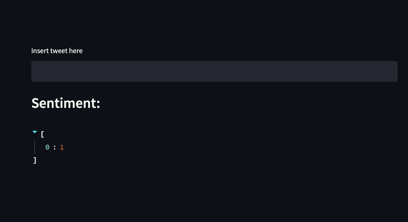
If you connect to http://54.146.192.225:8501, the External URL, you’ll be able to interact with the dashboard app:
All good, but we can do better and exploit TMUX to start a streaming session, so we can log out from the virtual machine and interact with the app without staying connected. Let’s install TMUX:
sudo apt-get tmux
and start a streaming session:
tmux new -s StreamlitSession
Now we can freely run Streamlit and the app will run within the tmux session:
You can leave the SSH shell by pressing Ctrl+B and aside press the key D. This combination will detach you from the tmux session and you’ll be able to log out from the SSH connection. If you want to stop the tmux session just reconnect to the machine and look for the PID of the running job
ps aux | grep streamlit
and kill the process with
kill PID NUMBER
At this stage, we can have a little review of the entire process. We can immediately point out some pros:
- The Git-DagsHub interface is easing our lives by providing a dedicated MLflow server and storage. This saves a lot of time and hassle, as we do not have to set up virtual machines or specific VPC permissions or infra (e.g. peerings) to allow the MLflow system to be shared across all our entire cloud tools
- If we are AWS-based MLflow provides a super simple interface to deal with our registered models. We do not need to worry about creating Dockerfiles or specific SageMaker codes
and some cons:
- We may not be AWS based. In this case, MLflow offers a great solution for Azure deployment but not for Google Cloud Platform. I tried to fill up this gap a little while ago but further work is needed to have a more seamless interface between MLflow model registry and GCP
- If you’d like to spin up this model to Heroku, DagsHub doesn’t currently offer any CI/CD interface with this deployment provider. Thus, you’d need to create a few more images (docker-compose) to have the registered model and the endpoint interface wrapped up by Heroku and hosted as custom images
- SageMaker endpoints cost! Before deploying your super ML model consider the chance of deploying a SageMaker Batch Transform job rather than an endpoint. Here is the GitHub issue request and links to the MLflow PRs that accommodate this Batch Transform request.
Thus, we need to consider future work from this starting point. First of all, we could find a suitable way to fill the gap between MLflow and other cloud providers (not Azure, not AWS). Additional help may come from Seldon. Seldon offers an MLflow interface to host and spin up models — regardless of some complications which may arise from Kubernetes. It is worth mentioning this very recent MLflow implementation, which is a new mlflow deployment controller, that could pave all the deployment roads on multiple Cloud platforms. Stay tuned, because I’ll try out to share with you something similar 🙂
It’s been a long tutorial but I think you’re satisfied with the final result. We learned a lot of things, so let’s do a recap:
- We learned how to create a simple model and log it to MLflow, how to authenticate to MLflow, and track our experiments. Key takeaways: implementing MLflow Python bits, authentication, tracking concept.
- We saw how to make our code more general, exploiting the functionality of the
sklearnpipeline and creating our custom transformers for dealing with data and have them part of a final training pipeline. - We learned how to deploy our best model to AWS. Firstly we registered the model to the MLflow registry, then we used MLflow sagemaker deployment schemes and set up AWS IAM roles.
- Finally, we created a frontend for our model with Streamlit and we learned how to set up an EC2 instance to accommodate this application.
I hope you enjoyed this tutorial and thanks for reading it.
Denial of responsibility! Techno Blender is an automatic aggregator of the all world’s media. In each content, the hyperlink to the primary source is specified. All trademarks belong to their rightful owners, all materials to their authors. If you are the owner of the content and do not want us to publish your materials, please contact us by email – [email protected]. The content will be deleted within 24 hours.